
Alternating optimization#
Many estimation problems considered in the manuscript rely on solving an optimization problem that involves \(d\) different blocks, of the form
where \(f:\mathcal{X}_1\times \ldots \times \mathcal{X}_{d} \mapsto \mathbb{R}_+\) is a nonnegative cost function and \(\mathcal{X}_k\) are Euclidean spaces embedded in \(\mathbb{R}^{n_k}\). Indeed, LRA models are multifactor: each block \(x_k\) may represent a factor matrix in a low-rank model. For instance, solving a rank \(r\) approximate NMF problem in the presence of Gaussian noise may result in the following two-block optimization problem
for a known data matrix \(Y\in\mathbb{R}^{n_1\times n_2}\). In this example, and in fact in most problems involving LRA, the cost has interesting blockwise properties. Here, the cost is not convex because of the product of variables, but it is block-convex, and often blockwise strongly convex in practice. This observation hints at the design of a class of convergent algorithms for computing solutions to LRA problems that update each block sequentially.
This section provides a brief overview of existing results on methods that update the blocks of variables in an alternative manner. These methods are clustered in two groups: Alternating Optimizations methods (AO) where the cost is exactly minimized with respect to each block alternatively, and Block Coordinate Descent methods (BCD) where the cost decreases with respect to each block alternatively. BCD methods considered here are all, in fact, particular cases of alternating MM algorithms. The literature on both AO and BCD is old and vast; I present mostly recent results of practical interest to the rest of the manuscript, but an interested reader should find in these recent references many acknowledgments of previous works. AO was especially intensively studied in the 1970s. This section is also similar to, and heavily inspired by, chapters 11 and 14 from the book of Amir Beck [Beck, 2017], and to Section 8.1.3 in the book of Nicolas Gillis [Gillis, 2020]. The book of Beck also constitutes a great introduction to convex optimization in general, which can be completed by the book of Dimitri Bertsekas [Bertsekas, 1999].
We build the rest of this section as follows. First, common assumptions are quickly recalled. Then AO and BCD are introduced sequentially, moving from the more general to the more specific results.
Summary of assumptions and convergence results#
This section collects useful assumptions for the convergence results of AO and BCD. The definitions of convexity, differentiability, Lipschitz-smoothness, and related optimization concepts are not recalled and can be found, for instance, in [Beck, 2017]. The shorthand notation \(x = (x_1,\ldots,x_d)\) is used.
Here is a list of the assumptions required for proving the convergence of AO and BCD:
(A0): \(f\) can be splitted as \( f(x) = f_0(x) + \sum_{k=1}^{d} r_k(x_k)\).
(A1): \(\mathcal{X}_k\) are closed convex sets.
(A2): \(f\) has bounded level sets \(I_f(z)=\{x | f(x) \leq z\}\).
(A3): \(f\) is proper, lower semicontinous.
(A4): \(f\) is convex.
(A5): \(f\) is continuous over its domain, that is, continuous strictly in the interior of the definition domain.
(A6): \(f\) is differentiable in the interior of its domain.
(A7): \(f\) is continuously differentiable.
(A8): \(f\) is globally Lipschitz-smooth.
(A9): \(f\) is block Lipschitz-smooth, meaning that the restrictions of function \(f\) on each block are Lipschitz-smooth.
(A10): \(f\) admits directional differentials defined at \(x\) along direction \(d\) as \(f'(x,d) = \underset{\lambda \to 0}{\lim\inf}\frac{f(x\lambda d) - f(x)}{\lambda}\) (notice that \(\lambda\) is positive). This includes nonsmooth functions such as the \(\ell_1\) norm.
(A11): The block updates \(\argmin{x_k\in\mathcal{X}_k} f(x_1,\ldots,x_k,\ldots,x_d)\) have a unique minimizer.
(A12(p)): \(f\) is block strictly quasiconvex with respect to \(p\) blocks. Quasiconvexity of the function \(f\) is equivalent to the assumption that any level set \(I_f(z)\) is convex.
(A13): \(f\) is non-increasing on the update path.
(A14): \(f\) is regular at the limit points of the algorithm sequence.
We use the notation (A9)(\(f\)) to denote, for instance, assumption (A9) applied on the maps \(f\). (A0) and (A4,A7)(\(f_0\)) mean that \(f\) can be split as \(f_0\) and separable maps \(r_k\), and that \(f_0\) is convex and differentiable on the interior of its domain. When an assumption, e.g., convexity, applies on a majorant \(u\) of \(f\), the notation (A4)(\(u\)) is used. Table List of convergence results summarizes the various convergence results for AO and BCD with their assumptions.
Reference |
Assumptions |
Result |
|---|---|---|
(A2,A3,A5,A11)(\(f\)) |
AO limit points are coordinatewise minimum |
|
(A1) (A0,A2,A3,A5,A11)(\(f\)) (A6)(\(f_0\)) (A3,A4)(\(r_k\)) |
AO limit points are stationary points |
|
(A0,A2,A3,A5)(\(f\)) (A4,A6)(\(f_0\)) (A3,A4)(\(r_k\)) |
AO limit points are stationary points |
|
(A1) (A3,A6,A11,A13)(\(f\)) |
AO limit points are stationary points |
|
(A1) (A3,A5)(\(f\)) |
\(d=2\) AO limit points are stationary points |
|
(A1) (A3,A5,A12(d-2))(\(f\)) |
AO limit points are stationary points |
|
(A1) (A2,A3,A10)(\(f\)) |
SUM sequence converges to a stationary point |
|
(A1) (A3,A10,A14)(\(f\)) (A11,A12(d))(\(u\)) |
BSUM limit points are stationary points |
|
(A1) (A2,A3,A10,A14)(\(f\)) (A11)(\(u\)) |
BSUM iterates converge to stationary points |
This section also relies on the concept of MM, already discussed in the context of EM in Nonnegative regressions: NNLS and NNKL. Providing an overview of MM in this manuscript would be out of scope; the reader is referred to the excellent survey article by Sun, Babu, and Palomar [Sun et al., 2017].
Note
Three assumptions often found in the numerical optimization literature,
a function is lower-semicontinuous,
a function is closed,
a function has closed level sets,
are equivalent when considering extended real-valued functions from an Euclidean space, see [Beck, 2017] Theorem 2.6. The results in the book by Beck use the terminology “closed”, but I prefer “lower-semicontinuous”, which is more clearly related to continuity.
Alternating Optimization#
AO, sometimes also called exact BCD, minimizes the cost function \(f\) sequentially for each block of variables, essentially performing cyclic updates
at iteration \(i+1\) and for the \(k\)-th block. It is immediate to observe that because the cost \(f\) is positive, and because each AO update diminishes the cost, the sequence of cost function values is always decreasing. Therefore, the AO algorithm converges, in cost, towards a positive value. Interesting questions, therefore, are not to know if the AO algorithm converges in cost, but rather:
Does AO converge in cost to a stationary point, and at what rate?
Are the sequences of iterates \(\{x^{(i)}_k\}_{k\leq d}\) converging towards a stationary point in the nonconvex case, or the global minimizer in the convex case, and at what rate?
A famous counter-example for the convergence of AO was proposed by Powell in 1973 [Powell, 1973]. This counter-example occurs because the minimization subproblems with respect to each block do not have a unique solution (A11) [Beck, 2017]. We will see below that most AO convergence guarantees rely on this assumption.
One may note the similarity with the assumptions for the convergence of MM to stationary points. For \(d=2\) blocks, single-block MM and AO are in fact equivalent [Sun et al., 2017]. Denoting
we get that
Two blocks AO is exactly the computation of, first, \(x_2(x_1^{(i)})\), and then the minimization of the majorant \(f(x_1,x_2(x_1^{(i)}))\). This majoration can be loose for arbitrary functions without inter-block regularity, which can intuitively explain the slow convergence discussed in different-flavours-of-convergence-of-ao-iterates.
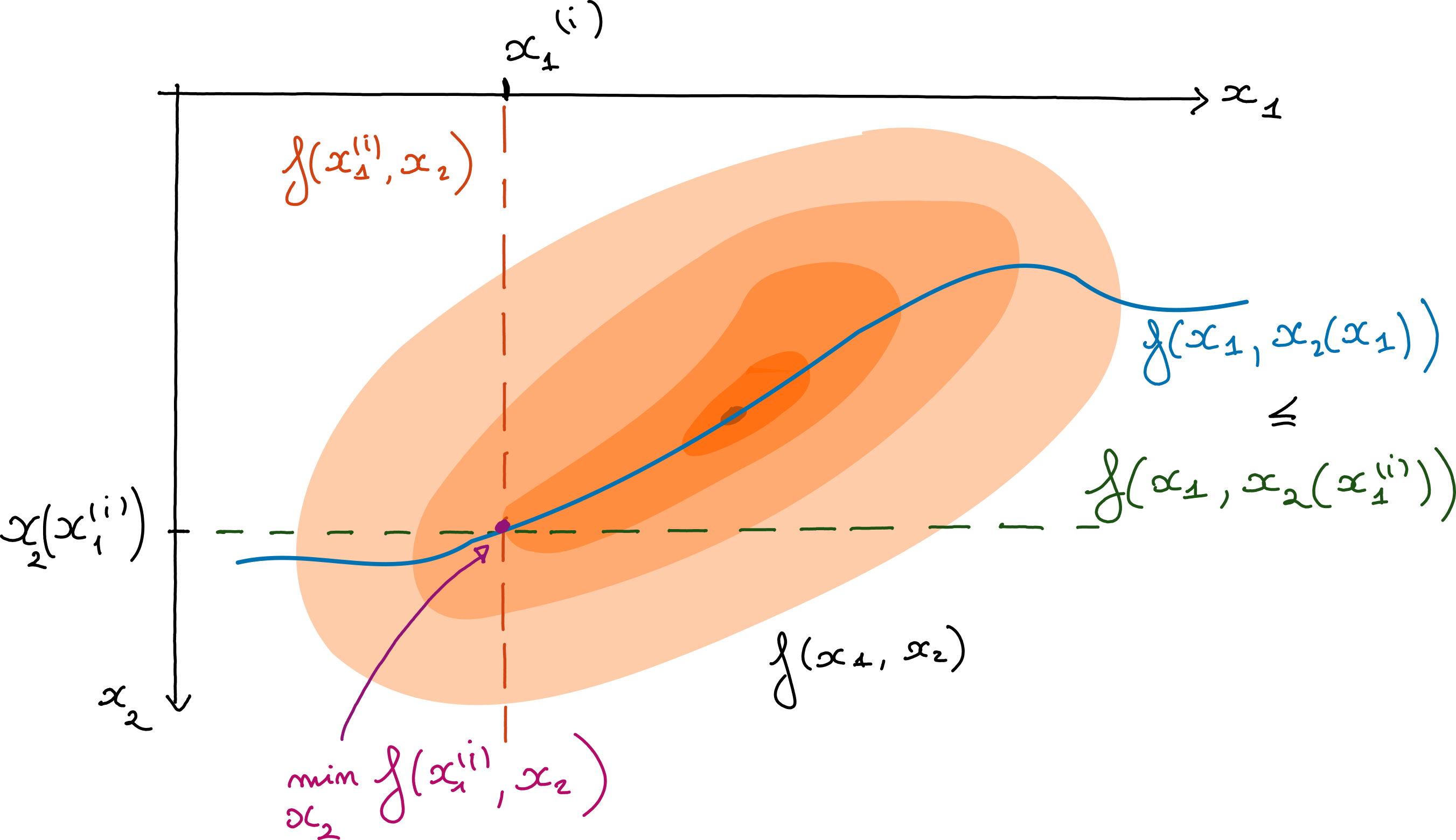
Fig. 21 AO seen as a MM technique. The colored surfaces represent level sets of the bivariate loss \(f(x_1,x_2)\). The horizontal dashed line is the loss function restricted to the line \(x_2 = x_2(x_1^{(i)})\) for some estimated \(x_1^{(i)}\) at iteration \(i\). Along this line the loss is always greater than the cost on the curve \(f(x_1, x_2(x_1))\) which is always optimal with respect to \(x_2\) for a fixed \(x_1\). The minimization of the loss along the horizontal dashed line yields one iteration of AO.#
Another immediate issue with AO is that, without additional assumptions, it may converge only to a coordinatewise minimum, namely a point at which the cost \(f(x)\) is minimal along each coordinate. Coordinate-wise minima are not necessarily stationary points, and Beck shows that this holds even when the cost is convex. The root of the problem is that the Fermat rule \(0\in\partial f\) does not decompose into separate conditions for each block, unlike the gradient for differentiable functions: it is always true that \(\nabla f = 0\) is equivalent to \(\forall k\leq d,~\frac{\partial}{\partial x_k} f = 0 \), but for non-differentiable functions, \(0\in\partial f\) only implies \(\forall k\leq d,~0\in\partial f_k\) while the converse is not true. This explains why most works on AO that consider nonsmooth costs introduce assumption (A0), additive separable nonsmooth regularizations \(r_i\) to a differentiable multi-block cost \(f_0\),
where \(f_0\) is proper, lower-semicontinuous, and continuously differentiable over its domain (it can be nonconvex), and functions \(r_k\) are proper, convex, lower-semicontinuous. A typical example where the constraints are nonsmooth and nonseparable is linear coupling constraints between variables; AO for these problems is bound to get stuck at a coordinatewise minimum, which may be irrelevant to the global optimization problem.
Different flavours of convergence of AO iterates#
Probably the most well-known result on the convergence of AO is due to Dimitry Bertsekas and was published in his book Nonlinear Programming in 1995 [Bertsekas, 1999]. There have been several iterations of his result, in particular to distinguish between convergence to coordinatewise minima and stationary points. Below is a summary of Bertsekas’s result and its variations.
Theorem 3 (Convergence of AO, nonconvex nonsmooth)
Assumptions (A2,A3,A5,A11)(\(f\))
Assume that the function \(f\) is proper, lower-semicontinuous, and continuous over its domain. Assume that each block update (6) has a unique solution. Assume also that the level sets of the function \(f\) are bounded. Then the sequence of AO iterates is bounded, and any limit point is a coordinatewise minimum.
From [Beck, 2017, Bertsekas, 1999]
As discussed above, the convergence to coordinatewise minima is of little use for nonsmooth functions, since they are not necessarily stationary points. Therefore, while this first result does not require differentiability, in practice it should be used with caution in a non-differentiable setup; hence the splitting of smooth and nonsmooth terms in this second theorem.
Theorem 4 (Convergence of AO, nonconvex smooth + separable convex nonsmooth)
Assumptions (A1) (A0,A2,A3,A5,A11)(\(f\)) (A6)(\(f_0\)) (A3,A4)(\(r_k\))
Assume that the function \(f\) is proper, lower-semicontinuous, and continuous over its domain. Assume that each block update (6) has a unique solution. Assume also that the level sets of the function \(f\) are bounded.
If moreover function \(f\) decomposes as \(f(x) = f_0(x) + \sum_{k\leq d} r_k(x_k)\) with \(r_k\) proper, lower-semicontious, continuous over its domain and convex, and \(f_0\) lower-semicontinuous, differentiable on the interior of a Cartesian product of closed convex sets, then any limit point of the AO iterates is a stationary point.
From [Beck, 2017]
There are two further versions of this result. First, one may want to relax the assumption that the block updates have unique solutions; this assumption can indeed be too strong in practical cases where convergence is yet observed. This assumption can be easily relaxed if the cost \(f\) is convex.
Theorem 5 (Convergence of AO, convex smooth + separable convex nonsmooth)
Assumptions (A0,A2,A3,A5)(\(f\)) (A4,A6)(\(f_0\)) (A3,A4)(\(r_k\))
Assume that the function \(f\) is proper and continuous over its domain. Assume also that the level sets of the function \(f\) are bounded.
If moreover function \(f\) decomposes as \(f(x) = f_0(x) + \sum_{k\leq d} r_k(x_k)\) with \(r_k\) proper, lower-semicontinuous, continuous over its domain and convex, and \(f_0\) continuously differentiable and convex, then any limit point of the AO iterates is a stationary point.
From [Beck, 2017]
A second version that applies in the nonconvex case discards the splitting and the boundness of the level sets assumptions. To obtain convergence to a stationary point, differentiability is required. The level set assumption is replaced by the requirement that along the block updates, the cost is non-increasing, a property resembling pseudo-convexity often used in earlier AO convergence proofs. This is actually the original result by Bertsekas.
Theorem 6 (Convergence of AO, nonconvex smooth)
Assumptions (A1) (A3,A6,A11,A13)(\(f\))
Assume that the function \(f\) is proper, lower-semicontinuous, and continuously differentiable over its domain, which is a Cartesian product of closed convex sets. Assume that each block update (6) has a unique solution.
Assume further that the cost is non-increasing in the interval
Then any limit point of the AO iterates is a stationary point.
From [Bertsekas, 1999]
It is important to note that the order of the AO block updates is not important in these results, as long as there exists an integer \(K\) such that each block is updated at least once in every \(K\) AO iterations [Gillis, 2020].
Convergence rate of AO
The convergence rate of the AO algorithm with arbitrarily many blocks is found in the book of Amir Beck [Beck, 2017]. AO converges sublinearly in the convex, Lipschitz-smooth plus separable convex nonsmooth case; in fact, AO has the same asymptotic convergence speed as first-order methods. Moreover, the convergence rate depends linearly on the Lipschitz constant \(L_{f_0}\) of the function \(f_0\), and therefore on the worst Lipschitz constant over all blocks. In practice, however, AO can be faster than BCD. An example of this phenomenon for gradient descent performed over \(\mathcal{X}_1 \times \ldots \times \mathcal{X}_d\) is discussed in Practical issues.
AO with \(d=2\) blocks#
An important special case is AO with two blocks. The convergence of AO with two blocks has been studied in the seminal paper of Grippo and Scriandrone [Grippo and Sciandrone, 2000].
Theorem 7 (Convergence of AO, \(d=2\), nonconvex smooth)
Assumptions (A1) (A3,A5)(\(f\))
Assume that the function \(f\) is continuously differentiable, and assume that the sets \(\mathcal{X}_1\) and \(\mathcal{X}_2\) are closed and convex sets. Then the limit points of the AO iterates are stationary points.
Notice how the assumptions for the two-block case are milder than in the general case. Compared to Theorem 6, the two-block case requires neither the uniqueness of block updates nor the monotonicity of the cost along the update path. The two-block case is useful when considering the convergence of alternating algorithms for models such as NMF or Dictionary Learning (DL).
Convergence rate of AO with two blocks
The convergence rate of AO with two blocks is still sublinear under convexity and separable nonsmoothness assumptions, but the constant is now proportional to the smallest Lipschitz constant of \(f_0\) for the two blocks, a sharp improvement with respect to the \(d>2\) blocks case [Beck, 2017]. Moreover, the function \(f_0\) need not be Lipschitz-smooth and may be differentiable only on an open set.
Extension of the two-blocks case#
Grippo and Scriandrone also provide a convergence result for \(d>2\) blocks based on blockwise strict quasiconvexity of the cost for \(d-2\) blocks and continuous differentiability of the cost.
Theorem 8 (Convergence of AO, block strictly quasiconvex, smooth)
Assumptions (A1) (A3,A5,A12(d-2))(\(f\))
Assume that the function \(f\) is continuously differentiable, and that the sets \(\mathcal{X}_k\) are closed and convex. Further assume that the function \(f\) is blockwise strictly quasiconvex with respect to \(d-2\) blocks. Then the limit points of the AO iterates are stationary points.
This result requires both blockwise strict quasiconvexity and the differentiability of the cost, and is weaker in that sense than the variants introduced above. Yet because it does not require the uniqueness of the block updates and does not require convexity with respect to all blocks, it can sometimes be applied in contexts where Theorem 4 cannot.
Block-coordinate descent#
AO is a simple framework for multiblock optimization problems, but its convergence guarantees can be hard to satisfy. In particular, computing the exact block updates and ensuring their uniqueness can be challenging. The convergence rate is also sublinear, and one may hope to find faster alternating algorithms. BCD is another algorithmic framework in which the blocks are updated sequentially (in any order), but each block update may only reduce the cost function value. The next sections introduce BCD frameworks based on the MM principle.
Successive upper-bound minimization#
The Successive Upper-bound Minimization framework (SUM), proposed by Razaviyayn, Hong, and Luo in 2013 [Razaviyayn et al., 2013], is an extension of the MM principle, in which the majorant must be continuous and have the same first-order derivative as the cost at the majoration point in all directions. This requirement is rather weak in practice, as many MM algorithms rely on Taylor expansions to build the majorants, in which case this tangent condition holds.
The SUM framework is simple to describe and essentially the same as the MM framework. Consider a single block function \(f(x)\).
At a given point \(x^{(i)}\), build a continuous majorant \(u(y,x^{(i)})\) of the cost \(f\), tight and tangent.
Compute \(x^{(i+1)}\) as a minimizer of the majorant \(u(y,x^{(i)})\) over \(y\).
Repeat 1. and 2. until convergence.
The convergence of SUM is simple to prove under mild assumptions.
Theorem 9 (Convergence of SUM, nonconvex nonsmooth)
Assumptions (A1) (A2,A3,A10)(\(f\))
Assume that the function \(f\) admits directional derivatives at all points, and that the set \(\mathcal{X}\) is closed and convex. Further assume that the majorant \(u\) in SUM satisfies the majoration conditions, namely it is tight, tangent in all directions, and upper-bounds the cost at all points. Then every limit point of the SUM iterates is a stationary point. If, further, the level set \(\{x| f(x)\leq f(x^{(0)}) \}\) is bounded, then the iterates converge to the set of stationary points.
From [Razaviyayn et al., 2013].
A typical use of the SUM framework is when the cost decomposes as \(f(x) = f_0(x) + r(x)\), with function \(f\) continuously differentiable and function \(r\) a proximable regularization with direction derivatives such as the \(\ell_1\) norm. Then SUM where \(f\) is majorized by a second-order Taylor expansion of \(f_0\) with an isotropic quadratic term is exactly a proximal gradient descent algorithm. SUM also covers the MU algorithm discussed in Nonnegative regressions: NNLS and NNKL. In general, the convergence rate of SUM is therefore at best sublinear.
The block successive upper-bound minimization framework#
The extension of SUM to a multiblock function is called Block SUM (BSUM) and is a generic framework that encompasses many other BCD algorithms, such as PALM [Bolte et al., 2014], under the hypothesis that the cost admits directional derivatives. BSUM is exactly the application of SUM sequentially over all blocks, in any order. Compared to SUM, BSUM requires additional assumptions for convergence, which come in two flavors. First, one may assume that the majorants are quasiconvex and that the block updates have unique solutions.
Theorem 10 (Convergence of BSUM, quasiconvex nonsmooth)
Assumptions (A1) (A3,A10,A14)(\(f\)) (A11,A12(d))(\(u\))
Assume that the function \(f\) admits directional derivatives at all points, and that the sets \(\mathcal{X}_k\) are closed and convex. Further assume that the majorants \(u\) in BSUM satisfy the majoration conditions for all blocks, namely the majorants are tight, tangent in all directions, and upper-bound the cost at all points. Additionally, assume that the majorants for each block are quasiconvex, and that the block updates have unique solutions.
Then every limit point of the BSUM iterates is a coordinatewise minimum. If, further, the cost is regular at all these limit points, then the limit points of the BSUM iterates are stationary points.
From [Razaviyayn et al., 2013].
A second version of this convergence result avoids the quasiconvexity assumption and shows convergence of the iterates, rather than of their limit points, towards the set of stationary points. It relies on the compacity of the level set \(I_f(x^{(0)})= \{x| f(x)\leq f(x^{(0)}) \}\) where \(x^{(0)}\) is the initialization of the BSUM iterates.
Theorem 11 (Convergence of BSUM, nonconvex nonsmooth)
Assumptions (A1) (A2,A3,A10,A14)(\(f\)) (A11)(\(u\))
Assume that the cost function \(f\) admits directional derivatives at all points, and that the sets \(\mathcal{X}_k\) are closed and convex. Further assume that the majorants \(u\) in BSUM satisfy the majoration conditions for all blocks, namely the majorants are tight, tangent in all directions, and upper-bound the cost at all points. Additionally, assume that the level set \(I_f(x^{0})\) is bounded, and that the block updates have unique solutions for at least \(d-1\) blocks. Further, assume that the cost is regular at all the stationary points.
Then the BSUM iterates converge to the set of stationary points.
From [Razaviyayn et al., 2013].
It is important to note that, as with AO, the BSUM framework assumes that the constraint sets are disjoint. In particular, BSUM cannot handle linear couplings between blocks of variables, and in fact, BSUM, like AO, is bound to fail in this setup.
The convergence rate of BSUM was studied in the convex case [Hong et al., 2017]. BSUM, PALM, and other similar first-order BCD algorithms have, in general, sublinear convergence rates, see also chapter 11 of the book of Beck [Beck, 2017].
BCD with extrapolation#
An important research direction to accelerate BCD algorithms is to leverage extrapolation of iterates, inspired by the seminal work of Nesterov on the fast gradient algorithm [Nesterov, 1983]. Going into the details of all the proposed extrapolated BCD methods would be out of scope. Instead, an interested reader will find below a list of a few useful works on this topic. These methods typically also have sublinear rates, but improved from \(\mathcal{O}(i^{-1})\) to \(\mathcal{O}(i^{-2})\) where \(i\) is the iteration index.
Alternating Proximal Gradient Descent (APGD) [Xu and Yin, 2013] is a general framework for alternating algorithms, that covers AO and PALM with extrapolation. APGD assumes that the cost is the sum of a strongly convex term (for AO) or Lipschitz smooth (for PALM with extrapolation) and separable convex nonsmooth regularizations. The originality lies in the general conditions with asymptotic rates and the extrapolation for PALM.
iPALM is an extension of PALM with extrapolation [Pock and Sabach, 2016]. It is similar to APGD but relaxes a condition on the monotonicity of the cost along the update path.
TITAN [Hien et al., 2023] is essentially the BSUM framework with extrapolation. TITAN combines ingredients from PALM, such as the Kurdyka-Łojasiewicz property, with heavy-ball acceleration. A downside of TITAN is that it introduces, among others, the nearly sufficiently decreasing property that may not be satisfied when the majorants are not strongly convex. This condition can be relaxed, provided other assumptions on the extrapolation parameters, by using the framework of mirror gradient descent to include the extrapolation term in the majorant definition [Hien et al., 2025].
Practical issues#
From the convergence properties summarized above, it is far from obvious whether AO or BCD should be preferred in practice. What’s more, AO and BCD are optimization frameworks, but their implementations can significantly affect performance. For BCD in particular, the order in which the blocks are visited and the number of times each block is updated before switching to a different block are important topics.
AO vs BCD vs approximate AO#
Let us discuss a concrete example of NMF with the Frobenius loss; see Low-rank matrix and tensor models and Nonnegative regressions: NNLS and NNKL for details on the NMF model and classical solvers. The solver we consider is HALS. Denoting \(W\) and \(H\) the two factors of the NMF \(Y\approx WH^T\), HALS can be seen as a BCD algorithm where the blocks are the columns of matrices \(W\) and \(H\). Each block update is computed in closed form.
The HALS updates for the columns of matrix \(H\) involve computing the quantities \(W^TW\) and \(W^TY\). In fact, in high-dimensional settings, these operations are the computational bottleneck of HALS. Because these quantities are independent of matrix \(H\), it is more efficient in terms of computation cost to update the columns of matrix \(H\) several times, sequentially, before switching to matrix \(W\). The number of times \(n_{inner}\) the columns of matrix \(H\) (and similarly for \(W\)) are updated is thus a hyperparameter of HALS. The outer iterations are incremented once both matrices have been updated.
If the number of inner iterations \(n_{inner}\) is set to a large number, the HALS algorithm is essentially an (approximate) AO algorithm, ANLS, solving the NNLS problem for matrices \(W\) and \(H\) alternatively. One may wonder if setting the number of inner iterations \(n_{inner}\) to a low number leads to a sharper decrease of the cost per outer iteration, meaning that BCD has an advantage over AO in terms of convergence speed, and if this translates into a computation time advantage as well. Let us test the performance of HALS with various inner iterations \(n_{inner}\) numerically in a noiseless setting. The HALS implementation is taken from tensorly.
import tensorly as tl
import numpy as np
from tensorly.solvers import hals_nnls
from time import perf_counter

def BCD_hals(Y,Winit,Hinit,n_inner,n_outer):
    W = np.copy(Winit)
    H = np.copy(Hinit)
    start = perf_counter()
    loss = []
    time = []

    for it in range(n_outer):
        # Update H
        UtM = W.T @ Y
        UtU = W.T @ W
        H = hals_nnls(UtM, UtU, V=H.T, n_iter_max=n_inner, tol=0).T

        # Update W
        VtM = H.T @ Y.T
        VtV = H.T @ H
        W = hals_nnls(VtM, VtV, V=W.T, n_iter_max=n_inner, tol=0).T

        loss.append(np.linalg.norm(Y - W@H.T,'fro')**2)
        time.append(perf_counter() - start)
    return W, H, loss, time


# Generate toy synthetic nonnegative tensor data
np.random.seed(0)
shape = [2000, 50]
rank = 3
Wtrue, Htrue = [np.random.rand(s, rank) for s in shape]
Y = Wtrue @ Htrue.T
Winit = np.random.rand(shape[0], rank)
Hinit = np.random.rand(shape[1], rank)
results = {}

for n_inner in [1, 2, 3, 5, 10, 20, 100]:
    West, Hest, loss, time_ = BCD_hals(Y, Winit=Winit, Hinit=Hinit, n_inner=n_inner, n_outer=100)
    results[n_inner] = (loss, time_)
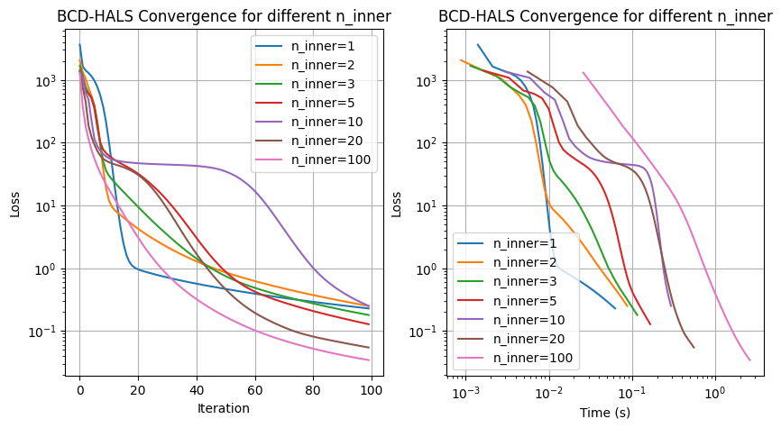
We may observe that:
Setting a large number of inner iterations leads to lower reconstruction error per outer iteration.
With respect to time, however, for a data matrix of size \(2000\) by \(50\), using one to five inner iterations leads to faster runtime to reach a high precision.
In this example, therefore, AO is a better strategy than BCD per outer iteration. We can only implement approximate AO, and its iterations are costly (solving the NNLS problem exactly requires many inner iterations of HALS); therefore, BCD should be used instead.
Note that this simulation is seeded. Running this experiment several times with different datasets and initializations yields different conclusions about the optimal number of inner iterations, both in terms of iterations and time. The dimensions of the input matrix are also an important factor, and for larger datasets (which makes this notebook slow to run and the whole manuscript, therefore, too slow to compile), setting the number of inner iterations higher can be beneficial. It can also be beneficial to run a different number of inner iterations for each matrix when their dimensions are vastly different; see, for instance, [Gillis and Glineur, 2012].
About continuous differentiability#
In this manuscript, we primarily use the squared Frobenius norm to measure discrepancies between the LRA model and the dataset. However, we also sometimes use \(\beta\)-divergences, and the KL-divergence in particular. It is then important to note that the KL-divergence is not differentiable at zero, and that, therefore, some of the results introduced above do not apply to the convergence of AO and BCD. Theorem 4, on the contrary, applies to KL-divergence loss since differentiability is only required in the interior of the domain of the smooth part \(f_0\) of the cost.
About compact sets and LRA#
One may object that many of the AO and BCD convergence results rely on the assumption that the sets \(\mathcal{X}_k\) are bounded or compact. In the context of LRA, due to scaling ambiguity, the block variables, which are typically the factors of the LRA model, do not belong to compact sets because these sets are unbounded. This problem is addressed in Gillis’s book on NMF, p. 267. His solution applies to most LRA models [Gillis, 2020]. In a nutshell, one may simply upper-bound the norms of the blocks with a large enough constant that depends on the data and the initialization. The trick also applies to guarantee that the level set \(\{x| f(x)\leq f(x^{(0)}) \}\) is compact as long as the cost is coercive.