Unrolled MU for data-driven NMF

Reference

[Kervazo et al., 2024] C. Kervazo, A. Chetoui and J. E. Cohen, “Deep unrolling of the multiplicative updates algorithm for blind source separation, with application to spectral unmixing”, EUSIPCO 2024. hal

[Kervazo and Cohen, 2025] C. Kervazo, J. E. Cohen, “Unrolled Multiplicative Updates for Nonnegative Matrix Factorization applied to Hyperspectral Unmixing, submitted pdf

Data-driven NMF principles

Data-driven NMF through regularization

Low-rank approximation models such as NMF are designed to perform unsupervised learning: given a data matrix \(Y\), their goal is to compute two possibly constrained matrices \(W,H\) such that \(Y\approx WH^T\). In practical applications, as discussed in Summary, however, performing LRA is not the final goal. The estimated factor matrices are instead further processed for a downstream task. These post-processing operations include clustering of the components, thresholding activations, or performing linear regression. Often, additional side information is available on the expected outcome of this post-processing. In the language of machine learning, we could say that this additional information takes the form of training data stored in a matrix \(M\).

A simple way to make use of this additional data \(M\) is to modify the LRA cost to incorporate this data. This procedure has been named “Supervised LRA” in the literature, see [Lock and Li, 2018] and references therein. For NMF, linear regression from a matrix \(W\) to additional data \(M\) can, for instance, drive the supervision task. The “supervised” NMF problem formulation is then given by

\[ \argmin{W\geq 0,\; H\geq 0,\; \theta} \mathcal{D}\left(Y, WH^T\right) + \lambda \|W - M\theta\|_F^2 \]

for a regularization hyperparameters \(\lambda>0\), a data fitting term \(\mathcal{D}\) such as the squared Frobenius norm \(\|Y-WH^T\|_F^2\), and regression parameters \(\theta\) trained jointly with the NMF factors.

One could argue that this approach does not really leverage training data to train a model in the way usually understood in supervised learning. Regression parameters \(\theta\) are learnt from scratch for each pair of data matrices \((Y,M)\). Matrix \(M\) must also be known at inference time.

A modification of this supervised LRA framework can be considered, in which the parameters \(\theta\) are shared across \(p\) LRA problems. In the above example of supervised NMF with linear regression, given a collection of data matrices \(\{(Y_i,M_i)\}_{i\leq p}\), parameters \(\theta\) are trained to reconstruct matrix \(M_i\) from the jointly estimated matrix \(W_i\):

\[ \argmin{\forall i \leq p,~ W_i\geq 0, H_i\geq 0, \theta}\sum_{i=1}^{p} \mathcal{D}\left(Y_i, W_iH_i^T\right) + \lambda \|W_i - M_i\theta\|_F^2. \]

Parameters \(\theta^\ast\), trained on the training dataset consisting of pairs \((Y_i,M_i)\), could then be used at inference time when only a single matrix \(Y\) is known to estimate matrix \(M:=\theta^\ast W^{\dagger}\) after obtaining matrix \(W\) with NMF, or by solving the NMF and the regression problem

\[ \argmin{W\geq 0, H\geq 0, M} \mathcal{D}\left(Y, WH\right) + \lambda \|W - M\theta^\ast\|_F^2. \]

We can still go further. In the formulations of supervised LRA above, while the post-processing parameters \(\theta\) and the parameter matrices are optimized jointly and move the solution of the supervised LRA problem away from the best low-rank approximation, the model applied to \(Y\) is still a low-rank approximation. Modern-day machine learning often relies on black-box models based on neural network architectures that lack strong inductive biases, such as bilinearity and low-rankness. Therefore, it is tempting to also train the model, in some sense, to better fit the training data. Formally, we may assume that the forward model is a map \(\mathcal{M}(W,H,\theta)\) and solve the optimization problem

(14)\[ \argmin{\forall i \leq p,~ W_i\geq 0, H_i\geq 0, \theta}\sum_{i=1}^{p} \mathcal{D}\left(Y_i, \mathcal{M}(W_i,H_i,\theta)\right) + \lambda \|W_i - M_i\theta\|_F^2. \]

An immediate issue with this formulation is that it is unclear how to even define such a map \(\mathcal{M}\) while ensuring that the matrices \(W\) and \(H\) remain interpretable in practice. Another issue is that computing the minimizers using first-order methods requires computing the derivatives of \(\mathcal{M}\) with respect to both the matrix \(W\) and the parameters \(\theta\), which can be challenging and time-consuming depending on the definition of the model \(\mathcal{M}\). As far as I know, supervised LRA models in the same form as Equation (14) have not been studied in the literature. Rather, a more convenient way of designing data-driven LRA models is through the lens of bilevel optimization.

Bilevel formulation for data-driven NMF

On top of the issues discussed above, a fundamental problem with supervised LRA as defined in Equation (14) is also the choice of hyperparameter \(\lambda\). Why should the user compromise between the quality of the forward pass of the model and the training of that model?

Bilevel formulations address the trade-off between model inference and parameter updates during training. There is, however, not a single canonical bilevel formulation for unrolling LRA. On the above example of supervised NMF, a naive formulation that separates the model computation (forward pass) and the actual training of the model (backward pass, i.e. updating model parameters \(\theta\) to reduce a training loss) writes

\[ \argmin{\theta,\; W} \sum_{i=1}^{p} \|M_i - W^\ast_i\theta\|_F^2 \quad \text{such that} \quad H_i^\ast, W_i^\ast = \argmin{W_i\geq 0, H_i\geq 0}\mathcal{D}(Y_i,W_iH_i^T). \]

Such a bilevel optimization problem is not particularly interesting because the two optimization problems are essentially decoupled and can be solved sequentially. We are back to simply post-processing the estimated parameter matrices of NMF. Following data-driven or task-driven dictionary learning [Mairal et al., 2011, Sprechmann et al., 2014], the symmetry between matrices \(W\) and \(H\) may be broken. We then solve a bilevel problem of the form

\[ \argmin{\theta} \sum_{i=1}^{p} \mathcal{L}(M_i, H_i^\ast(W), \theta) \quad \text{such that} \quad H_i^\ast(W) = \argmin{H_i\geq 0}\mathcal{D}(Y_i,WH_i^T). \]

Hence, the dictionary \(W\) is now trained to reduce the training loss \(\mathcal{L}\) while only the scores \(H_i\) are computed at the inner level. Updating matrix \(W\) means computing gradients through minimizers \(H_i^\ast(W)\), which is tractable analytically depending on the choice of the model, loss \(\mathcal{D}\), and in the presence of regularizations such as sparsity [Mairal et al., 2011]. It is, however, not obvious how to form these gradients for NMF.

The core idea of unrolling is to replace the inner optimization problem with a numerical algorithm that computes solutions to this problem:

\[ \argmin{\theta, \; W} \sum_{i=1}^{p} \mathcal{L}(M_i, H_i^\ast(W), \theta) \quad \text{such that} \quad H_i^\ast(W,\theta) = \mathcal{A}(Y_i,W,\theta), \]

where \(\mathcal{A}\) is a parametric algorithm to compute approximately a solution to NMF. Algorithm \(\mathcal{A}\) is chosen to be a fixed number of iterations of a truncated iterative algorithm. Note that the forward model / unrolled algorithm \(\mathcal{A}\) may depend on parameters \(\theta\) for greater flexibility.

One interesting property of unrolling is that even without training, the iterative algorithm that solves the problem, here NMF, typically works rather well for minimizing the supervision loss. In many problem instances, earlier contributions have addressed the problems at hand in a fully unsupervised manner. Therefore, finding a good initialization for the parameters \(\theta\) and the matrix \(W\) is often straightforward.

Unrolling the Multiplicative Updates algorithm

Existing unrolled NMF algorithms break the symmetry between matrices \(W\) and \(H\). Therefore, they are not well-suited to make use of training data in the form of pairs \((Y_i, (W^{gt}_i,H^{gt}_i))\), where \(W^{gt}_i\) and \(H^{gt}_i\) are ground-truth factors. A typical use case is source separation in remote sensing, where spectra and abundance maps may be provided alongside hyperspectral images; see (crossref) TODO. It is also possible to generate a synthetic training dataset in which one can produce both ground-truth matrices \(W\) and \(H\).

We therefore propose to formulate data-driven NMF where both matrices \(W\) and \(H\) are outputs of the parametric algorithm, solving

\[ \argmin{\theta} \sum_{i=1}^{p}\mathcal{L}(W_i^{gt}, H^{gt}_i, H_i(\theta),W_i(\theta)) \quad \text{such that} \quad \forall i\leq p,~ H_i(\theta),W_i(\theta) = \mathcal{A}(Y_i,\theta). \]

The main design choices for the unrolled algorithm are

• The (truncated) iterative algorithm \(\mathcal{A}\)

• The trained parameters \(\theta\).

In a series of works with Christophe Kervazo, we proposed unrolling a workhorse algorithm for NMF, the Multiplicative Updates algorithm; see Nonnegative Regressions: NNLS and NNKL for a detailed presentation. Other algorithms could be considered, but MU poses an interesting challenge: there are no obvious trainable parameters in the algorithm. For instance, the MU update for matrix \(W\) with Frobenius loss writes

\[ W \leftarrow W \ast \frac{YH}{WH^TH}. \]

Unrolling strategies typically train a stepsize or a linear operator in the log-prior (e.g. the finite difference operator). Strategies to unroll MU previously proposed by Nasser [ref Eldar] replace both matrix \(H\) and the cross product \(H^TH\) with trainable matrices. However, this strategy is not suited for an alternating procedure since the dependence on \(H\) is lost.

We proposed introducing trainable parameters that are multiplied elementwise with the updates. At iteration \(k\), the proposed Non-Adaptive Linearize MU (NALMU) is given by

\[ W^{k+1} = W^{k} \ast A^{k}_W \ast \frac{YH^k}{W^k{H^k}^TH^k} \text{ and } H^{k+1} \leftarrow H^k \ast A^k_H \ast \frac{Y^TW^{k+1}}{H^{k+1}{W^k}^TW^k}. \]

where \(A^{k}_W\) and \(A^{k}_H\) are iteration-dependant trainable matrices. There are two advantages to this choice:

1. Setting \(A^{k}_W\) and \(A^{k}_H\) to all-one matrices recovers MU. Therefore, the unrolled algorithm is easy to initialize, and we can understand how it differs from MU numerically.

2. We can prove that when updating a single matrix, say \(W\) with fixed \(H\), and with shared weights \(A^{k}_W\) across all iterations, the modified updates of NALMU can be obtained by a majorization minimization strategy using Jensen inequality, see Nonnegative Regressions: NNLS and NNKL, minimizing a modified cost function

\[ \| Y - WH^T \|_F^2 + \langle (W\ast A_W)H^T, Y \rangle, \]

where the data is compared to a masked NMF with factors \(W\ast A_W\) and \(H\). The trained parameters, therefore, act as weights emphasizing the reconstruction towards certain entries of \(W\).

Training NALMU

The supervision loss for NALMU is defined as

\[ \mathcal{L} = \sum_{i=1}^{p} \sum_{k=1}^{K} \nu_k \left(\ell_W(W_i^{k}(\theta), W_i^{gt}) + \ell_H(H_i^{k}(\theta), H_i^{gt})\right) \]

where \(W_i^{k}(\theta)\) and \(H_i^{k}(\theta)\) ar the estimated factors from algorithm \(\mathcal{A}\) after \(k\leq K\) iterations. Functions \(\ell_W\) and \(\ell_H\) are user-defined loss functions for the factor matrices, typically \(\ell_2\) norms or application-specific metrics such as the Spectral Angular Distance (SAD) used in remote sensing. Parameters \(\nu_k\) control how much the estimated factor after \(k\) iterations impacts the supervision loss; for instance, if only the final output of algorithm \(\mathcal{A}\) should match the ground-truth, then \(\nu_k = 0\) for any \(k<K\). Setting nontrivial values for parameters \(\nu_k\) avoids training issues such as vanishing gradients and is a common trick in the unrolling literature and more generally in deep learning.

The initial weights \(A_W\) and \(A_H\) can be set to one to start the learning phase from the MU algorithm. The number of truncated iterations \(K\) is, in general, set rather low compared to the maximum number of iterations used in MU. Typically, we choose \(K=25\). The training algorithm can be any classic optimizer in the deep learning community with default parameters. For instance, the AdamW optimizer with a learning rate of \(10^{-5}\) for 1000 epochs.

An issue with unrolled NMF is the scaling ambiguity, which makes the training less consistent. A simple solution we propose is to normalize the columns of the data matrices \(Y_i\) when appropriate, and to normalize the initial guesses for the factors accordingly. As a rule of thumb, normalisation in regularized and unrolled LRA can be tricky and should be designed depending on the application at hand.

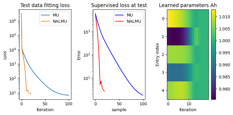
Toy example

Providing a full example of unrolled NMF in this manuscript is rather challenging, as the training of NALMU typically requires large computing resources. Rather, a minimal working example is implemented below to train NNLS (i.e., NMF with a fixed factor matrix, here \(W\)) on synthetic images generated from a noisy mixture. The goal of this toy experiment is to showcase one key feature of unrolled algorithms: they often provide a good reconstruction in much fewer iterations than the baseline algorithm.

import torch 
import matplotlib.pyplot as plt
# runs on CPU

# Hyperparameters
n = 5
m = 20
p = 500
sig = 0.1
K = 20
itermax = 1000
nu = torch.logspace(-7, 0, K)  # logspaced weights
#nu = torch.zeros(K)
#nu[K-1] = 1.0

# define training data
torch.manual_seed(2)
mu = 50*torch.rand(n, 1)
H = torch.randn(n, p) + mu  # H are generated around a true value mu
W = torch.rand(m, n)
Y = W@H + sig*torch.randn(m, p)

# define trainable parameters
Ah = torch.ones(n,K, requires_grad=True)
#Ah = torch.ones(n, requires_grad=True)

# define loss function
def loss_fn(Y, W, H):
    return torch.norm(Y - W@H)**2

# define MU updates
def MU_update(W, Y, Xinit, itermax=1000, Xgt=None):
    X = Xinit.clone().detach()
    WtW = W.T@W
    WtY = W.T@Y
    loss = [loss_fn(Y, W, X)]
    sup_loss = []
    for i in range(itermax):
        X = X*WtY/(WtW@X)
        loss.append(loss_fn(Y, W, X))  # can be optimized using stored quantities
        if Xgt is not None:
            sup_loss.append(torch.norm(X - Xgt)**2)
    return X, loss, sup_loss

# define unrolled MU updates
def NALMU(W, Y, Xinit, Ah, itermax=25, Xgt=None):
    X = Xinit.clone().detach()
    loss = [loss_fn(Y, W, X)]
    WtW = W.T@W
    WtY = W.T@Y
    Xs = []
    sup_loss = []
    for i in range(itermax):
        XAh = (X.T*Ah[:,i]).T
        #XAh = (X.T*Ah).T
        X = XAh*WtY/(WtW@X)
        Xs.append(X)
        loss.append(loss_fn(Y, W, X))  # can be optimized using stored quantities
        if Xgt is not None:
            supl = torch.norm(X - Xgt)**2
            sup_loss.append(supl.detach().numpy())
    return X, Xs, loss, sup_loss

# define optimizer
optimizer = torch.optim.Adam([Ah], lr=1e-2)   # using the Adam optimizer for simplicity

# Training
for epoch in range(500):
    optimizer.zero_grad()
    Hinit = torch.ones(n, p)
    H_est, Hs, _, _ = NALMU(W, Y, Hinit, Ah, itermax=K)
    loss = sum([nu[i]*torch.norm(Hs[i] - H)**2 for i in range(K)])  # weighted loss
    loss.backward()
    optimizer.step()
    if epoch % 10 == 0:
        print(f'Epoch {epoch}, Loss: {loss.item()}')

Show code cell output

Hide code cell output

Epoch 0, Loss: 10260.6171875
Epoch 10, Loss: 5403.9921875
Epoch 20, Loss: 1963.2296142578125
Epoch 30, Loss: 911.77392578125
Epoch 40, Loss: 466.202392578125

Epoch 50, Loss: 468.9923400878906
Epoch 60, Loss: 427.2074279785156
Epoch 70, Loss: 396.94952392578125
Epoch 80, Loss: 395.76837158203125
Epoch 90, Loss: 391.06500244140625

Epoch 100, Loss: 390.44451904296875
Epoch 110, Loss: 389.88873291015625
Epoch 120, Loss: 389.4041442871094
Epoch 130, Loss: 389.0443115234375
Epoch 140, Loss: 388.7633972167969

Epoch 150, Loss: 388.5315246582031
Epoch 160, Loss: 388.326904296875
Epoch 170, Loss: 388.1423034667969
Epoch 180, Loss: 387.97662353515625
Epoch 190, Loss: 387.82635498046875

Epoch 200, Loss: 387.6884460449219
Epoch 210, Loss: 387.5619201660156
Epoch 220, Loss: 387.444580078125
Epoch 230, Loss: 387.3362731933594
Epoch 240, Loss: 387.2344970703125

Epoch 250, Loss: 387.13970947265625
Epoch 260, Loss: 387.0508728027344
Epoch 270, Loss: 386.96807861328125
Epoch 280, Loss: 386.8887634277344
Epoch 290, Loss: 386.81402587890625

Epoch 300, Loss: 386.7436218261719
Epoch 310, Loss: 386.6759033203125
Epoch 320, Loss: 386.611572265625
Epoch 330, Loss: 386.5509338378906
Epoch 340, Loss: 386.492431640625

Epoch 350, Loss: 386.4364013671875
Epoch 360, Loss: 386.38262939453125
Epoch 370, Loss: 386.33123779296875
Epoch 380, Loss: 386.28173828125
Epoch 390, Loss: 386.23443603515625

Epoch 400, Loss: 386.1883544921875
Epoch 410, Loss: 386.1440734863281
Epoch 420, Loss: 386.10107421875
Epoch 430, Loss: 386.059814453125
Epoch 440, Loss: 386.019287109375

Epoch 450, Loss: 385.98046875
Epoch 460, Loss: 385.94281005859375
Epoch 470, Loss: 385.9061279296875
Epoch 480, Loss: 385.87017822265625
Epoch 490, Loss: 385.83514404296875

Show code cell source

Hide code cell source

# Test time!
p_test = 40
Htest = mu+torch.rand(n, p_test)
Ytest = W@Htest + sig*torch.randn(m, p_test)

H_NALMU, _, loss_NALMU, sup_loss_NALMU = NALMU(W, Ytest, torch.ones(n, p_test), Ah, itermax=K, Xgt=Htest)
H_MU, loss_MU, sup_loss_MU = MU_update(W, Ytest, torch.ones(n, p_test), itermax=5*K, Xgt=Htest)

# PLotting errors for MU and showing line with NALMU error after K iterations
fig, ax = plt.subplots(1,3, figsize=(8,4))
ax[0].semilogy(loss_MU)
ax[0].semilogy([loss_NALMU[i].detach().numpy() for i in range(len(loss_NALMU))])
ax[0].set_title('Test data fitting loss')
ax[0].set_xlabel('Iteration')
ax[0].set_ylabel('Loss')
ax[0].legend(['MU', 'NALMU'])

# Plot error bars for each sample
ax[1].semilogy(sup_loss_MU, 'b-')
ax[1].semilogy(sup_loss_NALMU, 'r-')
ax[1].set_title('Supervised loss at test')
ax[1].set_xlabel('sample')
ax[1].set_ylabel('Error')
ax[1].legend(['MU', 'NALMU'])

# Showing matrix Ah as an image
ax[2].imshow(Ah.detach().numpy(), aspect='auto')
ax[2].set_title('Learned parameters Ah')
ax[2].set_xlabel('Iteration')
ax[2].set_ylabel('Entry index')
#colorbar
ax[2].figure.colorbar(ax[2].images[0], ax=ax[2])
plt.tight_layout()
plt.show()

A few lessons to learn from this toy experiment:

• The choice of the \(\nu_k\) values greatly affect how far the weights \(A_W\) are from one. With the proposed choice (logarithmically spaced values in \([10^{-7}, 1]\)), the weights in the last layers are barely updated. Try setting all \(\nu_k\) to zero except the last one: the result is reversed, and the overall performance of NALMU decreases!

• Tied weights (when \(A_W\) does not depend on the iteration index) do not perform well in this example. This can be checked by changing the definition of \(A_W\) and updating the NALMU rule accordingly. In particular, NALMU with tied weights has difficulty reducing the NMF loss \(\|Y-WH^T\|^2\) over iterations.

• Unrolling algorithms is tricky in practice, and one needs to toy with the various hyperparameters and design choices.