
Implicit regularization in rLRA#
Reference
[Cohen and Leplat, 2025] J. E. Cohen, V. Leplat, “Efficient Algorithms for Regularized Nonnegative Scale-invariant Low-rank Approximation Models”, SIAM Journal of Mathematics on Data Science, 2025 [arxiv]
Consider the ridge NMF problem with Frobenius loss:
with \(M\in\mathbb{R}_{+}^{m_1\times m_2}\) and the nonnegative rank is \(r\).
Such a ridge-regularized model could be preferred by a user on the basis of ridge-regression: avoiding overfitting (in the case of NMF, this would translate as choosing a particular solution with low variance) or improving the numerical stability of the optimization algorithm (the optimization problem is strictly bi-convex when \(\lambda_i>0\)).
It turns out that, maybe surprisingly at first, the ridge-regularized NMF problem is equivalent (in the sense that the minimizers are related by a trivial mapping) to a variant of the nuclear-norm low-rank sensing problem with nonnegativity constraints,
This second formulation is insightful in many ways.
The regularization in the second, implicit formulation, takes the form of a group-sparse regularization of the rank-one terms in NMF. Without nonnegativity constraints, this constraint is exactly the nuclear norm of the low-rank matrix \(X_1X_2^T\). The ridge penalty on each factor matrix, therefore, implies rank-minimization implicitly.
Tuning each parameter \(\lambda_1\) and \(\lambda_2\) individually yields counterintuitive results. For instance, when \(\lambda_1\) is much larger than \(\lambda_2\), the regularization on the first factor \(X_1\) is not stronger than on the second factor \(X_2\). Only the product of the two regularization hyperparameters governs the regularization intensity.
In the work conducted with Valentin Leplat [Cohen and Leplat, 2025], we generalize this observation for a large class of regularized LRA models, namely Homogeneous Regularized Scale-Invariant models (HRSI), that account for many LRA models regularized with homogeneous positive-definite regularizations such as any \(\ell_p\) norm. The implicit rank-selection effect observed for ridge regularization is shown to be due to the scale-ambiguity of LRA models, and therefore pertains to most \(\ell_p\) norms. We provide the main theoretical result below, and provide more examples, namely \(\ell_1\)-\(\ell_1\) and \(\ell_1\)-\(\ell_2\) regularizations.
We present numerical simulations in the next section, along with algorithm-oriented concerns, such as leveraging scale-invariance to optimally balance the factors to minimize regularization, which provably allows one to escape the so-called “scaling swamp” [Papalexakis et al., 2013].
Scale invariance main result#
While the scale of the factor matrices leaves the low-rank approximation intact, namely \(X_1X_2^T\) and \(X_1\Lambda \Lambda^{-1}X_2^T\) are equivalent low-rank representations for any nonzero diagonal matrix \(\Lambda\), implicit regularization in LRA essentially occurs because the regularizations are not invariant with respect to such a balancing of columns and rows of the factor matrices. Solving for the optimal scales in rLRA modifies the penalization. Further, the optimal scales are determined by the homogeneity degree of the regularizations and the value of the regularization hyperparameters, and essentially balance the rank-one components.
In what follows, we first introduce the general framework of HRSI, and then derive the main result that relates scale-invariance with implicit regularization.
Homogeneous Regularized Scale-Invariant models#
Consider the following optimization problem
where \(f\) is a continuous map from the Cartesian product \(\times_{i=1}^{n} \mathbb{R}^{m_i\times r} \cap \text{dom}(g_i)\) to \(\mathbb{R}_+\), \(\{\mu_i\}_{i\leq n}\) is a set of positive regularization hyperparameters, and \(\{g_i\}_{i\leq n}\) is a set of lower semicontinous regularization maps from \(\mathbb{R}^{m_i}\) to \(\mathbb{R}_+\). We assume that the total cost is coercive, ensuring the existence of a minimizer. Furthermore, we assume the following assumptions hold:
A1: The function \(f\) is invariant to columnwise scaling of the parameter matrices. For any sequence of positive diagonal matrices \(\{\Lambda_i\}_{i\leq n}\),
\[ f(\{X_i\Lambda_i\}_{i\leq n}) = f(\{X_i\}_{i\leq n})\;\;\text{if}\; \prod_{i=1}^{n}\Lambda_i = I_r, \; \Lambda_i>0. \]In other words, scaling any two columns \(X_{i_1}[:,q]\) and \(X_{i_2}[:,q]\) inversely proportionally has no effect on the value of \(f\).
A2: Each regularization function \(g_i\) is positive and homogeneous of degree \(p_i\), that is for all \(i\leq n\) there exists \(p_i>0\) such that for any \(\lambda > 0\) and any \(x\in \mathbb{R}^{m_i}\),
\[ g_i(\lambda x) = \lambda^{p_i} g_i(x). \]This property holds in particular for any \(\ell_p^p\) norm.
A3: Each function \(g_i\) is positive-definite, meaning that for any \(i\leq n\), \(g_i(x)=0\) if and only if \(x\) is null.
We refer to the optimization problem (8) with assumptions A1, A2, and A3, the Homogeneous Regularized Scale-Invariant problem (HRSI).
HRSI is quite general and encompasses many instances of regularized LRA problems. Specifically, ridge NMF is an HRSI problem with \(f(\{X_i\}_{i\leq n})= \|M - X_1X_2^T\|_F^2\), \(g_1(x) = \|x\|^2_2 + \eta_{\mathbb{R}_+^{m_1}}(x)\) and \(g_2(x) = \|x\|^2_2 + \eta_{\mathbb{R}_+^{m_2}}(x)\).
Solutions to HRSI also solve an implicit regularized problem, and are balanced#
We proved the following result in [Cohen and Leplat, 2025], relying on an identity for the geometric mean.
Theorem 12 (HRSI solutions characterization and implicit equivalent formulation)
If \(\mu_i>0\) for all \(i\), any solution \(\{X_i^\ast\}_{i\leq n}\) to the HRSI problem (8) under assumptions A1, A2 and A3 satisfies
for all \(i\leq n\) and \(q\leq r\), where
Moreover, the solutions to the HRSI problem are, up to scaling, solutions to the implicit HRSI problem
where \(\tilde{\mu} = \left(\prod_{i=1}^{n}(p_i\mu_i)^{\frac{1}{p_i}} \right)^{\frac{1}{\sum_{i=1}^{n} \frac{1}{p_i}}}\left(\sum_{i=1}^{n}\frac{1}{p_i}\right).\)
From this theorem, we observe that
Only the product of regularization hyperparameters impacts the regularity of the solution.
The sum of columnwise regularization on the factor matrices in the explicit formulation becomes a product of regularizations in the implicit formulation, yielding group-sparsity on the rank-one components.
At optimality, the scales of the components must satisfy the balancing condition \(p_i\mu_ig_i(X_i^{\ast}[:,q])=\beta_q\). This means, in particular, that LRA models regularized with homogeneous functions do not suffer from scale ambiguity.
Special cases with \(\ell_1\) and \(\ell_2\) regularizations#
To make our main result Theorem 12 more explicit, let us instantiate the implicit HRSI formulation and the optimal scales for a couple of classical problems in rLRA. Based on the observation that only the product of regularization hyperparameters matters, the same regularization hyperparameter is used for all factor matrices.
Ridge-regularized nonnegative CPD#
Define the ridge nCPD formally as the optimization problem
The implicit HRSI problem shows that ridge-regularization yields a componentwise group-sparsity implicit regularization,
where tensors \(\mathcal{L}_q\) are rank-one tensors \(X_1[:,q]\otimes X_2[:,q] \otimes X_3[:,q]\). We experimentally validate in the experiments subsection that tuning the regularization hyperparameter \(\mu\) indeed helps us to select the rank of the nCPD factorization automatically. Moreover, the optimal solution of ridge nCPD verifies the balancing equation
This balancing identity will be used in the experiments subsection to refine the iterations of an iterative optimization algorithm to solve ridge nCPD.
Sparse NMF L1-L1#
Another interesting case of an implicit regularization effect concerns the (double) sparse NMF model
Intuitively, a practitioner using sparse NMF with \(\ell_1\) penalizations on both factors would expect sparse entries in both matrices, leveraging the usual behavior of the \(\ell_1\) norm in regression problems. The implicit formulation
shows that, while both factors are indeed penalized to be sparse, there is another group-sparse effect that prunes entire components. The problem with this formulation is that both effects (elementwise sparsity and componentwise sparsity) are not controlled individually but rather by the same regularization hyperparameter. This yields unexpected component pruning as shown in the simulation below with mixtures of Gaussians. It is also unclear from the implicit formulation whether both factors will be sparse elementwise.
import numpy as np
import tensorly as tl
import matplotlib
import matplotlib.pyplot as plt

# Generating toy image
n1 = 30
n2 = 40
r = 3
sig = 0.2  # 0.15 # 0.05

# Components will be Gaussian distributions, here is the macro to generate them
def gauss(x, m, sig, thresh=0.1):
    # max is 1
    out = np.exp(-(x-m)**2/sig**2)
    out[out < thresh] = 0
    return out

# Generating the data as a mixture of separable Gaussians
x = np.linspace(0, n1-1, n1) # 1D abcisse
y = np.linspace(0, n2-1, n2)
W = np.zeros([n1, r])
W[:,0] = gauss(x, 5, 3)
W[:,1] = gauss(x, 15, 5)
W[:,2] = gauss(x, 25, 10)
H = np.zeros([n2, r])
H[:, 0] = gauss(y, 10, 5)
H[:, 1] = gauss(y, 20, 6)
H[:, 2] = gauss(y, 25, 5)
trueNMF = (None, [W, H])

Y = W@H.T  # NMF model
rng = np.random.default_rng(1246)
Yn = Y + sig*rng.random((n1, n2))  # corruption with gaussian noise

# initialization
W0 = 0*W + 0.5*rng.random(W.shape)
H0 = 0*H + 0.5*rng.random(H.shape)

# Storing output factors for various regularization in dictionaries
We = dict()
He = dict()

# Chose the grid values for the hyperparameter
lambset = [0, 0.05, 0.1, 0.15, 0.2, 0.3, 0.4, 0.6, 0.7, 0.75, 0.78, 0.8, 1, 1.2, 1.5, 2, 3, 4, 5, 5.2, 6, 20]

import copy
for lamb in lambset:
    # Computing the sparse NMF with tensorly (the algorithm is HALS, which is the state of the art for this problem)
    out = tl.decomposition.non_negative_parafac_hals(Yn, r, sparsity_coefficients=[lamb, lamb], init=copy.deepcopy((None, [W0, H0])))
    # Estimated factors
    We[lamb] = out[1][0]
    He[lamb] = out[1][1]
    # Set estimates as new initialization for the next iteration (warm start)
    W0 = We[lamb]
    H0 = He[lamb]

    # rescale We so that when a column of W is 0, so is the corresponding column of H
    norms = tl.max(We[lamb], axis=0)
    for q in range(r):
        if norms[q] > 1e-8:
            We[lamb][:, q] = We[lamb][:, q]/norms[q]
            He[lamb][:, q] = He[lamb][:, q]*norms[q]
        else:
            We[lamb][:, q] = We[lamb][:, q]*0
            He[lamb][:, q] = He[lamb][:, q]*0
Observe in particular that the sparsity level of the components does not evolve smoothly with the regularization hyperparameter. Components vanish brutally at \(\mu=0.75\) and \(\mu=5.2\).
The sparse NMF using \(\ell_1\)-\(\ell_2\) regularization#
The explicit \(\ell_1\)-\(\ell_2\) sparse NMF model writes
The implicit HRSI formulation of sparse NMF can be easily derived:
where the mixed matrix norm is defined as \(\|L_q\|_{1,2} = \sqrt{\sum_{j} \left( \sum_i L_q[i,j] \right)^2} \) and we used the identity
that holds for any two vectors \(x\) and \(y\). One may observe that the implicit regularization acts as a group-LASSO norm on the rows of the rank-one components, effectively enforcing sparsity elementwise in the factor matrix \(X_1\). The group-LASSO effect on the rank-one components still appears, however, in the implicit regularization, and similarly to the \(\ell_1\)-\(\ell_1\) case, the two effects may occur simultaneously.
It is still open to fully characterize the link between the regularized formulation and the constrained formulation
Interestingly, Marmin, Goulard, and Févotte show equivalence between the constrained formulation and the implicit HRSI formulation of sparse NMF, hinting towards the equivalence between the three formulations [Marmin et al., 2023].
Balanced and non-Euclidean algorithms for regularized LRA#
In our work with Valentin Leplat, in addition to the theoretical analysis of HRSI discussed in Implicit regularization in rLRA, we tackle a more practical problem. We observe, both numerically and theoretically, the existence of scaling swamps that considerably slow the convergence of alternating algorithms. Can the balancing equation \(p_i\mu_ig_i(X_i^{\ast}[:,q]) = \beta_q\) be leveraged to escape these swamps?
In what follows, we first show the existence of scaling swamps in a toy problem numerically ([Cohen and Leplat, 2025] formally proves the sublinear convergence rate of ALS for this problem). A simulation then shows the rank-selection capabilities of ridge nCPD, along with the importance of balancing.
Scaling swamps#
In the tensor decomposition literature, swamps refer to many consecutive iterations of optimization algorithms in which the cost function remains nearly constant while the parameters change significantly. This phenomenon occurs for many algorithms and is conjectured to be due to the ill-posedness of tensor LRA [Hillar and Lim, 2013], [Comon et al., 2009], [Mohlenkamp, 2019], [Vermeylen et al., 2025].
Another kind of swamp was observed by Papalexakis and Sidiropoulos [Papalexakis et al., 2016] for \(\ell_1\)-\(\ell_1\) sparse NMF. It is called a scaling-swamp because, as in traditional swamps, the cost improves very slowly over many iterations. Unlike in swamps from the tensor decomposition literature, however, the cost does not decrease any faster after a certain number of iterations, and scaling swamps also occur in matrix factorization problems such as NMF, even though the low-rank manifold is closed.
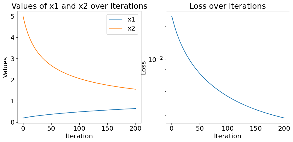
We can construct a simple numerical example in one dimension in which the ALS algorithm is provably slow. Consider the loss function
where \(x_1\) and \(x_2\) are real values and the regularization hyperparameter \(\lambda\) and the data \(y\) are positive real values.
Using a perturbation analysis, it can be observed that the ALS algorithm, whose updates at iteration \(k+1\) are given by
has a convergence rate for the iterates asymptotically close to \(1-4\lambda/y\), which is arbitrarily close to one (sublinear convergence) for small regularizations. The following numerical simulation shows that scaling swamps are more pronounced when regularization is small relative to the data magnitude.
from matplotlib import axes
import numpy as np
import matplotlib.pyplot as plt

# A barebone implementation of the ALS (Alternating Least Squares) algorithm
def ALS(y,x1,x2, lamb, itermax=200):
    loss = [(y - x1*x2)**2 + lamb * (x1**2 + x2**2)]
    x1_store = [x1]
    x2_store = [x2]
    for k in range(itermax):
        x1 = x2*y/(x2**2+lamb)
        x2 = x1*y/(x1**2+lamb)
        loss.append((y - x1*x2)**2 + lamb * (x1**2 + x2**2))
        x1_store.append(x1)
        x2_store.append(x2)
    return x1, x2, loss, x1_store, x2_store

# Example usage, you can play with the values of y and lamb !
y = 1
lamb = 0.001

# Initialization
x1 = 0.2
x2 = 5

# Prints and Plots
x1, x2, loss, x1store, x2store = ALS(y, x1, x2, lamb)
print("After 200 iterations:")
print(f"x1: {x1}, x2: {x2}, Optimal values: {np.sqrt(y-lamb)}")
print(f"Loss: {loss[-1]}, Optimal loss: {(y-np.sqrt(y-lamb))**2+ lamb * 2 * (y-lamb)}")
After 200 iterations:
x1: 0.642558430874947, x2: 1.5525184957484308, Optimal values: 0.999499874937461
Loss: 0.0028290328046436134, Optimal loss: 0.00199825012507818
Interestingly, the toy problem (9) has a simple closed form solution that can be obtained by optimally balancing the two scalar values \(x_1\) and \(x_2\) as defined in Theorem 12, namely
Then the optimal solution is simply (up to sign ambiguities) \(x_1=x_2=\sqrt{y-\lambda}\).
This suggests that balancing the estimates optimally before, after, or within an optimization algorithm solving HRSI could help avoid the scaling swamp phenomenon. We explore here only the balancing of initialization and/or outputs of an algorithm for simplicity.
Balancing initial or final estimates of an algorithm is a straightforward operation using Theorem 12. First, compute the columnwise geometric mean
Then scale all columns such that their regularization is exactly \(\frac{1}{p_i\mu_i}\beta_q\). For the problem of ridge-regularized nCPD, this amounts to performing for all \(i\) in \(\{1,2,3\}\) the balancing procedure
An example barebone implementation is shown below.
import matplotlib.pyplot as plt
import tensorly as tl
from copy import deepcopy
from tensorly.solvers.penalizations import scale_factors_fro

def optimal_balancing(factors):
    rank = factors[0].shape[1]
    beta = []
    for q in range(rank):
        beta.append(tl.prod([tl.norm(factor[:,q]) ** (1 / 3) for factor in factors]))
    balanced_factors = []
    for i in range(len(factors)):
        balanced_factor = factors[i].copy()
        for q in range(rank):
            balanced_factor[:, q] =  factors[i][:, q] * beta[q] / tl.norm(factors[i][:, q])
        balanced_factors.append(balanced_factor)
    return balanced_factors
The simulation below illustrates the importance of balancing initial (and sometimes final) estimates. In [Cohen and Leplat, 2025], we also show that balancing at every outer iteration in the HALS algorithm further improves the convergence speed empirically.
Recall the ridge-regularized nCPD problem
The reader can play around with the regularization value: high values lead to more component pruning, but the effect of balancing is less pronounced; low values lead to no component pruning, but the importance of balancing is more visible, even after the optimization algorithm has converged.
Also note that balancing only optimizes the factor scales with respect to the regularization terms. To scale the factors also according to the data fitting term and therefore start the algorithm at the best scaled position, it can be useful to scale the initial guess by solving the polynomial minimization problem
which amounts to evaluating the cost at all the positive roots of the polynomial
# Example usage of the optimal_balancing function
rank = 3
dims = [10, 11, 12]
ndims = len(dims)
noise = 0.1
itermax = 100

# Regularization hyperparameter
ridge_reg = 0.1

# Create random factors for a 3-way tensor decomposition
np.random.seed(22)  # For reproducibility
true_factors = [tl.tensor(np.random.rand(dims[i], rank)) for i in range(ndims)]

# Creating the data (from factors or balanced factors, it leads to the same result)
CPtensor = tl.cp_tensor.CPTensor(([10**(-i) for i in range(ndims)], true_factors))
data = CPtensor.to_tensor() + noise * tl.tensor(np.random.randn(*dims))  # Adding some noise

# Initialization
rank_e = rank + 3  # overestimating rank for initialization
init = [10**(-i) * tl.tensor(np.random.rand(dims[i], rank_e)) for i in range(ndims)]
CPinit = tl.cp_tensor.CPTensor((None, init))

# Optimal scaling of the initialization
t_init_unscaled = CPinit.to_tensor()
CPinit_scaled, scale = scale_factors_fro(CPinit, data, [ridge_reg]*ndims, [0]*ndims, nonnegative=True)
init_scaled = CPinit_scaled.factors

# Balancing the unscaled initialization factors
balanced_init = optimal_balancing(init)
CPinit_balanced = tl.cp_tensor.CPTensor((None, balanced_init))

# Balancing the scaled initialization factors
balanced_scaled_init = optimal_balancing(init_scaled)
CPinit_scaled_balanced = tl.cp_tensor.CPTensor((None, balanced_scaled_init))
Optimal scaling factors: 5.290233987029234
Initial factors:
Factor 0: shape (10, 6), norm 4.299994791774854
Factor 1: shape (11, 6), norm 0.4074799825930501
Factor 2: shape (12, 6), norm 0.04968474562511675

Scaled factors:
Factor 0: shape (10, 6), norm 22.74797859149603
Factor 1: shape (11, 6), norm 2.1556644529478346
Factor 2: shape (12, 6), norm 0.2628439299428947

Balanced factors:
Factor 0: shape (10, 6), norm 0.43822144179578987
Factor 1: shape (11, 6), norm 0.43822144179579
Factor 2: shape (12, 6), norm 0.4382214417957899

Balanced scaled factors:
Factor 0: shape (10, 6), norm 2.3182939652330408
Factor 1: shape (11, 6), norm 2.3182939652330408
Factor 2: shape (12, 6), norm 2.3182939652330408
# Fetching the loss values with callback
callback_loss = []
def callback(factors, unnormalized_rec_errors):
    loss = (unnormalized_rec_errors**2)/2 + sum([ridge_reg*tl.norm(factors[1][i])**2 for i in range(3)])
    callback_loss.append(loss)

# Running nonnegative CP decomposition with various balancing/scaling setups
from tensorly.decomposition import non_negative_parafac_hals

CPe = non_negative_parafac_hals(data, rank_e, n_iter_max=itermax, tol=0, init=deepcopy(CPinit), verbose=False, ridge_coefficients=ridge_reg, callback=callback)
loss = np.copy(callback_loss)

callback_loss = []
CPe_scaled = non_negative_parafac_hals(data, rank_e, n_iter_max=itermax, tol=0, init=deepcopy(CPinit_scaled), verbose=False, ridge_coefficients=ridge_reg, callback=callback)
loss_scaled = np.copy(callback_loss)

callback_loss = []
CPe_balanced = non_negative_parafac_hals(data, rank_e, n_iter_max=itermax, tol=0, init=deepcopy(CPinit_balanced), verbose=False, ridge_coefficients=ridge_reg, callback=callback)
loss_balanced = np.copy(callback_loss)

callback_loss = []
CPe_scaled_balanced = non_negative_parafac_hals(data, rank_e, n_iter_max=itermax, tol=0, init=deepcopy(CPinit_scaled_balanced), verbose=False, ridge_coefficients=ridge_reg, callback=callback)
loss_scaled_balanced = callback_loss
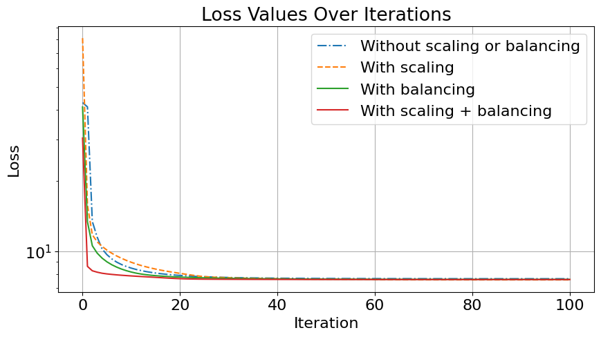
We can also look at the loss function with and without balancing of the final estimates to observe that balancing reduces the final error slightly, and the effect is more prononced for the output of algorithms that did not scale and balance the initial guess.
# Balancing the final estimated factors
CPe_fbalance = tl.cp_tensor.CPTensor((None, optimal_balancing(CPe.factors)))
CPe_scaled_fbalance = tl.cp_tensor.CPTensor((None, optimal_balancing(CPe_scaled.factors)))
CPe_balanced_fbalance = tl.cp_tensor.CPTensor((None, optimal_balancing(CPe_balanced.factors)))
CPe_scaled_balanced_fbalance = tl.cp_tensor.CPTensor((None, optimal_balancing(CPe_scaled_balanced.factors)))

def loss(data, CPestim, ridge_reg):
    regs = sum([ridge_reg * tl.norm(factor) ** 2 for factor in CPestim.factors])
    return 0.5 * (tl.norm(data - CPestim.to_tensor()) ** 2) + regs
Final Loss values before | after rebalancing:
Without balancing or scaling:
7.640703504963442 | 7.640136375087222
With scaling:
7.558884490291016 | 7.558384623717727
With balancing:
7.58741959225447 | 7.5869139361472975
With scaling and balancing:
7.581340753614703 | 7.58123879130162