
Nonnegative PARAFAC2#
Reference
[Cohen and Bro, 2018] J. E. Cohen, R. Bro, “Nonnegative PARAFAC2, a flexible coupling approach”, LVA/ICA 2018, arXiv:1802.05035
[Roald et al., 2021] M. Roald, C. Schenker, J. E. Cohen, E. Acar, “PARAFAC2 AO-ADMM: Constraints in all modes”, EUSIPCO2021, arxiv
[Roald et al., 2022] M. Roald, C. Schenker, V. D. Calhoun, T. Adali, R. Bro, J. E. Cohen, E. Acar, “An AO-ADMM approach to constraining PARAFAC2 on all modes”, SIAM Journal of Mathematics on Data Science, 2022. arxiv code SIMODS
Why Nonnegative PARAFAC2#
The PARAFAC2 model is often used in applications such as Liquid/Gas Chromatography Mass Spectroscopy (LCMS and GCMS, respectively) to extract mass spectra and time elution profiles for various experimental setups. The mixture of interest is injected into a long tube where the various chemical compounds glide at different speeds, and therefore reach the end of the tube at different times. By measuring the mass spectrum at the output of the tube with a mass spectrometer, one may acquire spectra at various time instants. One acquisition, therefore, yields a data matrix with intensities collected at various coordinates (mass-to-charge (m/z) x time). Repeating this acquisition several times for different chemical compounds yields a tensor dataset, with the third dimension indexing the experiments. An example GCMS dataset is available below, with different wine samples from various producers measured individually. The full dataset is described in [Ballabio et al., 2008].
One interesting feature of this dataset, visible in the top-right plot, is that the time elution profiles shift slightly with the experiment index.
Formally, given a collection of mass spectra over time \(X[:,:,k]\) where \(k\leq K\) stands for the experiment index, supposing elution profiles and mass spectra can be extracted from each experiment using a low-rank approximation, and further supposing that these components are shared across all experiments, estimating these components amounts to computing
that is by computing a CPD from the data tensor \(X\). The factors bear physical meaning (mass spectra, elution time profiles, and experiment contribution); it is reasonable to impose nonnegativity on all factors.
However, in practice, as observed in this dataset, the injection of chemical compounds into the chromatography system is done manually, which impacts the elution time. Elution time may also fluctuate due to other experimental conditions, such as temperature. Therefore, the time profiles of components \(B\) are slightly modified across experiments indexed by \(k\). As discussed in PARAFAC2 and variants, further constraints are required to link the resulting \(B_k\) matrices, and PARAFAC2 ensure in particular that
The columns of factors \(B_k\) are transformed similarly (the same transformation matrix \(P_k\) applies to each column \(B[:,q]\)).
The cross product of the \(B_k\) factors is constant.
A technical difficulty in applying PARAFAC2 to GCMS data is designing an optimization algorithm that allows for nonnegativity constraints on the \(B_k\) matrices. Indeed, the classical algorithm to fit PARAFAC2 proposed by Kiers and Bro [Kiers et al., 1999] relies on the reparameterization \(B_k = P_kB\). It can be summarized as follows:
Compute the optimal \(P_k\) matrices by solving \(K\) orthogonal Procrustes problems.
Compute the CP decomposition of the tensor obtained by stacking \(X[:,:,k]P_k\).
Loop the first two steps until convergence
The matrices \(B_k\) do not appear explicitly in this algorithm, and therefore, we need to rethink the optimization procedure to include these constraints.
Formalisation of the Nonnegative PARAFAC2 problem#
In our first work with Rasmus Bro, we proposed to use a flexible constraint formulation for the Nonnegative PARAFAC2 [Cohen and Bro, 2018]. While this work had a good impact on the chemometrics community, it relies on a relaxation of the PARAFAC2 constraint. It is, however, possible to use the AO-ADMM framework discussed in Constrained coupled matrix and tensor factorization to design an alternating iterative algorithm that solves the nonnegative PARAFAC2 problem. The core idea is to introduce a “PARAFAC2 constraint” on the matrices \(B_k\) that imposes that their cross products are constant. A collection of matrices \(\{B_k\}_{k\leq K}\) satisfies the PARAFAC2 constraint if for all \(k\leq K\), \(B_k^TB_k\) is constant. In that case we write that \(\{B_k\}_{k\leq K}\in\mathcal{C}_{\text{P2}}\).
Nonnegative PARAFAC2 then boils down to the optimization problem
This problem can be handled by AO-ADMM with splitting, provided we can project onto the set of sets of matrices satisfying the PARAFAC2 constraint. We explore this projection next.
Projection on the PARAFAC2 constraint#
A full understanding of the projection under the PARAFAC2 constraint has yet to be reached, and it remains an active research topic. It connects with Riemmanian geometry and optimization, but has not been studied in this literature as such, to the best of my knowledge.
In the work conducted with Marie Roald and co-authors, we used an empirical approach to this projection, relying on a few mathematical observations. First, notice that if a set \(\{ B_k\}_{k\leq K}\) satisfies the PARAFAC2 constraint, it can be represented as points on the orbit
Projection on the PARAFAC2 constraint therefore means finding a matrix \(B\) such that the total distance between each point \(B_k\) and the orbit \(\mathcal{O}(B)\) is as small as possible:
The distance \(d\) we propose to use is the Euclidean distance to the closest point \(P_kB\) on \(\mathcal{O}(B)\) to \(B_k\), that is
Projection on the PARAFAC2 constraint, therefore, boils down to solving
From the point of view of algorithm design, we seek a procedure to compute exact solutions to the problem (13) and plug them into the AO-ADMM algorithm. Maybe surprisingly, the following simple alternating algorithm typically converges in a few iterations:
Compute orthogonal matrices \(P_k\) solving \(K\) orthogonal Procrustes problems.
Compute the geodesic mean \(B\) as \(\argmin{B} \sum_{k} \|P_k^TB_k-B\|_F^2 = \frac{1}{K}\sum_{k} P_k^TB_k \).
We can observe the procedure’s fast convergence empirically in the experiment below.
# Hyperparameters
dims = [10,10,5] # Dimensions of the tensor X
rank = 3 # Rank of the factorization
# Generate a collection of (nonnegative) matrices Bk randomly
Bks = [np.random.rand(dims[1],rank) for _ in range(dims[2])]
def project_parafac2(Bks, itermax=10):
B = sum(Bks) / len(Bks) # Initial guess as the mean of the input matrices
cost = [sum([np.linalg.norm(Bks[i] - B)**2 for i in range(len(Bks))])] # Initial cost
Pks = [np.eye(0) for _ in range(len(Bks))] # Initialize Pk matrices
for _ in range(itermax):
# Solve for Pk rotation matrices
for i in range(len(Bks)):
# Project each matrix Bk onto the PARAFAC2 constraints
U,s,V = np.linalg.svd(Bks[i]@B.T)
Pks[i] = U @ V
# Update B matrix as the mean
B = sum([Pks[i].T @ Bks[i] for i in range(len(Bks))]) / len(Bks)
# Recompute the cost
cost.append(sum([np.linalg.norm(Bks[i] - Pks[i] @ B)**2 for i in range(len(Bks))]))
print(f"Iteration {_+1}, Cost: {cost[-1]:.8f}")
return B, Pks, cost
out = project_parafac2(Bks, itermax=5)
Iteration 1, Cost: 2.21972701
Iteration 2, Cost: 2.17235400
Iteration 3, Cost: 2.17233334
Iteration 4, Cost: 2.17233331
Iteration 5, Cost: 2.17233331
The convergence speed of this alternating optimization algorithm is suspiciously fast, and we suspect that there may exist a similar procedure that converges in a single iteration, or at least a theoretical analysis guaranteeing the fast convergence of this heuristic projection. What is known for now is that this alternating algorithm converges to the solution of the problem, as a two-block alternating optimization with exact and unique solutions to each subproblem, see Alternating optimization.
Nonnegative PARAFAC2 for GCMS data#
We may now compute PARAFAC2 with and without nonnegativity constraints on the time elution mode. The AO-ADMM implementation of PARAFAC2 with constraints is found in the matcouply package[Roald, 2023], developed by Marie Roald at Simula (Norway) during her PhD thesis. For PARAFAC2 without nonnegativity on the second mode (but with nonnegativity on the first mode to avoid sign ambiguities), we use the implementation available in tensorly, which uses reparameterization and relies on the CP decomposition.
import matcouply as mcl
from matcouply.decomposition import parafac2_aoadmm
from tensorly.decomposition import parafac2
# With nonnegativity constraint
cmf_nn, diagnostics_nn = parafac2_aoadmm(
tensor, 3, n_iter_max=200, non_negative=True, verbose=False, return_errors=True, tol=1e-9, random_state=5
)
weightsnn, (Ann, B_isnn, Cnn) = cmf_nn
# tensorly unconstrained PARAFAC2
pf2, rec_err = parafac2(
tensor, 3, n_iter_max=200, return_errors=True, nn_modes=[0], random_state=0, tol=1e-9, verbose=False
)
weights, (A, B, C), P_is = pf2
B_is = [P_i @ B for P_i in P_is]
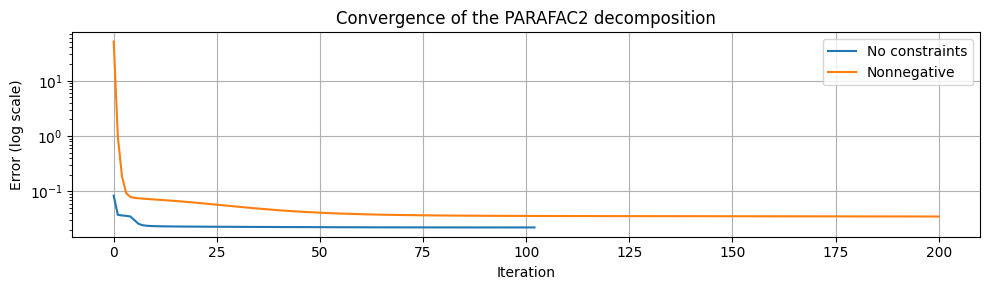
One may observe that the nonnegative PARAFAC2 model can recover elution peaks that overlap significantly with the baseline. Without nonnegativity constraints, the extracted elution profiles are somewhat mixed, and the baseline is found in all three components.
In a collaboration with Marie Roald, Carla Schenker, and Evrim Acar (SimulaMet, Oslo), we have extended the proposed algorithms for nonnegative PARAFAC2 to other constraints [Roald et al., 2022]. The algorithm works similarly by projecting onto the PARAFAC2 constraint and applying the proximity operator of the constraints to the \(B_k\) matrices, after splitting.