
Low-rank matrix and tensor models#
Low-rank models are important tools in both unsupervised and supervised machine learning, signal processing, and more generally in applied mathematics. They are also the main mathematical object studied in this manuscript. This section briefly introduces matrix, and tensor, Low-Rank Approximations (LRA). A solid background in linear algebra is required. Some of the material presented in the following sections has been covered in more detail in the book chapter I wrote with Pierre Comon and Rasmus Bro [Cohen et al., 2023]. The book of Golub and Van Loan provides a complete description of matrix low-rank models [Golub and Van Loan, 1989]. The recent book of Grey Ballard and Tammy Kolda provides a deeper introduction to tensor decompositions, with a focus on computational aspects [Ballard and Kolda, 2025].
Matrix low-rank factorizations and approximations#
There are at least two important ways in which a low-rank factorization of an \(n_1\) by \(n_2\) real-valued matrix \(M\) can be understood.
As a linear dimensionality reduction technique
Consider that matrix \(M\) is a collection of \(n_2\) vectors in \(\mathbb{R}^{n_1}\). A low-rank model describes the information contained in matrix \(M\) if and only if these \(n_2\) vectors belong to a smaller subspace of dimension \(r\leq n_1\). A low-rank model is therefore a linear dimensionality reduction technique. Dimensionality reduction is at the heart of both signal processing and machine learning, as it offers a compact representation of the input matrix that can be used to either compress the data or to mine information in an unsupervised manner by identifying an important set of variables.
Mathematically, a low-rank factorization of matrix \(M\) may be written as
Matrix \(U\) encodes a basis of the low-dimensional subspace spanning the columns of matrix \(M\), and \(V^T[:,j]\) is the vector of coordinates of each column \(M[:,j]\) in this basis. If the subspace dimension \(r\) is minimal, that is, there is no smaller subspace containing the \(n_2\) columns of \(M\), then the dimension \(r\) is called the rank of matrix \(M\) and is denoted \(\rank{M}\). Notice that if \(n_1\geq n_2\), then one may always reduce the dimension of the data by projecting on the column space spanned by the \(n_2\) columns. Therefore, this linear dimensionality-reduction interpretation is perhaps more meaningful when \(n_1 < n_2\). However, formally, the low-rank model reduces the dimension of the data whenever \(r\leq \min(n_1,n_2)\).
The computation of matrix \(U\) and coefficients \(V\) from the data matrix \(M\) can be performed using Singular Value Decomposition (SVD). Algorithms for the SVD rely on either QR decomposition or related tools from linear algebra; see the excellent book of Golub and Van Loan [Golub and Van Loan, 1989], and are implemented in the widely distributed LAPACK software [Anderson et al., 1999].
When the data matrix \(M\) is centered, the (truncated) SVD returns a particular low-rank factorization (approximation) of the data matrix, known as the Principal Component Analysis (PCA). PCA is a cornerstone of unsupervised machine learning, used not only for dimensionality reduction but also for mining information from high dimensional dataset; see Fig. 7 for an illustration, and low-rank-approximations for a discussion on approximations.
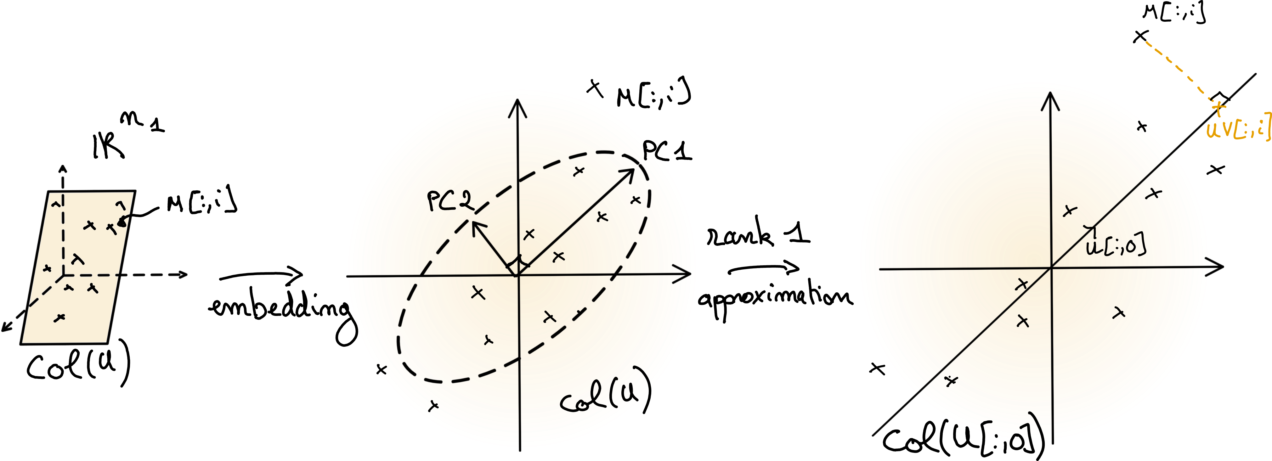
Fig. 7 Illustration of Principal Component Analysis. The centered data matrix \(M\) lies in a low-dimensional subspace \(col(U)\). If the orthogonal matrix \(U\) is computed from the data matrix \(M\), then the columns of \(U\) are the (unscaled) principal components. A low-rank approximation is obtained by projecting the data points on a subset of the principal components, here on the first component.#
As a factorization into a sum of rank-one matrices
Another equivalent description views low-rank models as decompositions of the matrix \(M\) into a sum of rank-one matrices. Formally, for a given integer \(r\leq \min(n_1,n_2)\),
The roles of matrices \(U\) and \(V\), often called factor matrices, are symmetric. Both factor matrices contain representations of rank-one terms \(M_q := U[:,q]V^T[q,:]\) such that \(M = \sum_{q=1}^{r} M_q\). Note that for fixed dimensions \(n_1\) and \(n_2\), rank-one matrices are simply the set \(\mathcal{M}_1\) of outer products of any two nonzero vectors,
The rank of matrix \(M\) is the smallest number of terms \(r\) such that the decomposition into rank-one terms exists. The two definitions of the rank above are equivalent. If \(M=UV^T\), then, equivalently, \(M[i,j] = \sum_{q=1}^{r} U[i,q]V[j,q]\).
The decomposition of a matrix as the sum of rank-one matrices can be understood as an atomic decomposition, where the dictionary is the set of rank-one matrices \(\mathcal{M}(n_1,n_2)\). The rank of a matrix is nonnegative and bounded above: any matrix \(M\) can be exactly described as a sum of rank-one matrices with at most \(\min(n_1,n_2)\) terms. Therefore, the rank of a matrix is one possible measure of matrix complexity: rank-one matrices are simple because they can be described with few parameters (a single atom), while full-rank matrices are the most complicated. In this interpretation, low-rank matrices where \(\rank{M}\ll \min(n_1,n_2)\) are especially interesting because, while they live in the ambient space \(\mathbb{R}^{n_1\times n_2}\), they can be summarized with only \(r\) atoms, described by \((n_1+n_2)r\) parameters.
The point of view of low-rank models as a decomposition into a minimal sum of rank-one terms establishes a clear link between inverse problems and LRA. It is also powerful when considering extensions of the notion of matrix rank to tensors.
Note
There are several other equivalent definitions of the rank for matrices that are widely used. An important definition is the dimension of the row-space or the column-space of a matrix \(M\), both of which are in fact equal in dimension.
Low-rank approximations#
In most practical applications of interest to this manuscript, the data matrices are not exactly low-rank. Instead, these data matrices are well approximated by low-rank matrices. A specific LRA is determined by the loss function, often the squared Euclidean distance, the input data matrix, and the rank of the approximation. A rank \(r\) approximation of a data matrix \(M\), in the Euclidean distance, can be formulated as an optimization problem
where \(\|M-N\|^2_F = \sum_{i,j} \left(M[i,j]-N[i,j]\right)^2\) is the (squared) Frobenius norm of the difference \(M-N\), with \(N\) the low-rank approximation of data matrix \(M\).
A different formulation of LRA is obtained if the approximation matrix is parameterized by two factor matrices \(U\) and \(V\),
a formulation often coined as the Burer-Montero factorization [Burer and Monteiro, 2003].
Note that the exact low-rank factorization problem may also be written with a similar formalism,
The Frobenius norm is the most widely used distance metric for LRA, as it yields a closed-form solution. Indeed, let \(M = ASB^T\) be the SVD of the matrix \( M\). Then the following result [Eckart and Young, 1936] shows that \(U=A\) and \(V^T = SB^T\) is optimal in the least squares sense.
Theorem 1 (SVD solves LRA with Frobenius norm (Eckart-Young theorem))
Assume data matrix \(M\) admits the singular value decomposition \(M = ASB^T\). Then the optimization problem
admits the truncated SVD as a solution, \(N^\ast = A[:,:r] S[:r,:r] B^T[:r,:]\). The solution is unique if the \(r\)-th singular value of \(M\) has multiplicity one. The residual error is then exactly \(\sum_{q=r+1}^{\min(n_1,n_2)}S[q,q]^2 \).
The Eckart-Young theorem is a remarkable and incredibly useful result in linear algebra, as LRA in Frobenius norm is one of the few nonconvex problems that admit a closed-form solution that can be computed efficiently. The same result holds (with a different residual) if the squared Frobenius norm is replaced by the spectral norm, but in general, the truncated SVD is not the solution to LRA with arbitrary loss functions. Another loss function often encountered in LRA is the KL-divergence discussed in NNKL problem definition.
Why are data matrices often (approximately) low-rank#
After many years of research in signal processing and machine learning, I have observed an intriguing yet recurring phenomenon: data matrices encountered in various applications are often approximately low-rank. While there is probably no general explanation for this phenomenon, here are a few (non-orthogonal) reasons why this can happen.
“Nice” latent variable models are of low-rank [Udell and Townsend, 2019], meaning that for a large catalogue of generative models, the resulting data matrix can be well approximated (in entry-wise error) by a low-rank matrix.
The entries of a rank-one matrix are samples of a separable map in two variables,
\[ f(x,y) = f_1(x)f_2(y). \]Separable maps are ubiquitous in physics since they allow for simple descriptions of multivariate functions.
Low-rank models \(M=UV^T\) can be seen as linear source separation models. The rank of the LRA is then the number of underlying sources. Matrix \(U\) contains columnwise the templates for the sources, and matrix \(V\) contains the mixing coefficients for these sources in the data. Nonlinearities, measurement noise, and missing data corrupt the low-rank data matrix. Many physical processes can be described this way, see examples in audio and hyperspectral image processing in Applications of rLRA: summary.
The second and third explanations also imply that in many applications, the factor matrices bear physical meaning: the practitionners ask of LRA for source separation to return good approximations of the underlying true factor matrices \(U\) and \(V\). There are two important questions to answer regarding the estimation of the factor matrices:
Is the model essentially identifiable, i.e., does equality of two low-rank models \(M= U_1V_1^T = U_2V_2^T\) implies equality of the factors up to trivial ambiguities ?
Is the estimation of factor matrices robust in the presence of noise?
Note
Trivial ambiguities in LRA are the scaling ambiguity, \(ab^T=\frac{1}{\lambda}a\lambda b^T\), and the permutation ambiguity \(UV^T=U\Pi\Pi^TV^T\) for any nonzero scalar \(\lambda\) and any permutation matrix \(\Pi\). These ambiguities arise from representing rank-one matrices as outer products but are not inherent to the atomic decomposition; the same atoms are used by two essentially equivalent low-rank factorizations. Essential uniqueness, meaning uniqueness up to permutations and scalings, is therefore considered.
The answer to the first question is negative: if \(U_1V_1^T = U_2V_2^T\) with the same rank for both models, then one may only assume that the two bases describe the same subspace, and are therefore related by an invertible transformation \(Q\in\mathbb{R}^{r\times r}\) such that \(U_1 = U_2Q\). This poses a fundamental problem for applications of LRA in source separation, as essential identifiability (or at least guarantees on the set of LRA solutions) is required to interpret the output of LRA algorithms as approximations to the ground-truth factor matrices. The rest of this section is therefore devoted to introducing further matrix and tensor decomposition models that enjoy identifiability conditions.
The answer to the second question is well understood in the context of matrix low-rank approximations in the Frobenius norm: the robustness of LRA is directly related to the conditioning number of the data matrix.
Note
The algorithmic development for LRA is only briefly described in this section. Two other sections in the manuscript are dedicated to numerical optimization: Nonnegative regressions: NNLS and NNKL and Alternating optimization.
Nonnegative Matrix Factorization#
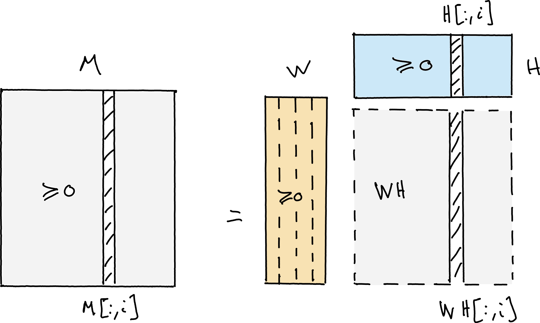
Fig. 8 Nonnegative Matrix Factorization (NMF) writes an elementwise nonnegative matrix \(M\) as the product of two elementwise nonnegative matrices \(W\) and \(H\) with respectively fewer columns and rows than \(M\).#
One possible route to make LRA parameters identifiable is to impose constraints on them. A constraint that is physically meaningful in many applications is nonnegativity. It applies naturally when factor matrices represent relative concentrations, spectral templates, images, probabilities, user ratings, energy, and other nonnegative physical quantities. The exact NMF model can be formulated as
Unlike unconstrained low-rank approximation, exact and approximate NMF do not admit, in general, closed-form solutions, although the best rank-one approximation may be obtained in closed form as discussed in Best nonnegative rank-one approximations. Computing (approximate) NMF amounts to solving an optimization problem. For instance, with the squared Frobenius norm, rank \(r\) approximate NMF computes
Computing exact NMF is an NP-hard problem [Vavasis, 2010]. There exist many strategies, many of which are based on alternating optimization, as discussed in Alternating optimization, and, to the best of my knowledge, there is no single best method for computing exact or approximate NMF for all datasets. An algorithm that provides reasonably good performance across a large set of problems is Hierarchical Alternating Least Squares (HALS); see Nonnegative regressions: NNLS and NNKL and Alternating optimization for a detailed description.
Another difficulty with NMF, compared to unconstrained LRA, is determining the approximation rank. With LRA, one may simply compute the full SVD of the input matrix and truncate according to the distribution of the singular values. Dropping orthogonality implies that the deflation strategy of truncated SVD does not transfer to NMF, and in fact, no deflation strategy exists for NMF that is as simple and general as truncated SVD. In practice, the rank is often guessed by the user, or several approximate NMF models are computed with various ranks, and the best model is kept. The nonnegative rank of a matrix is defined as the minimal integer \(r\) such that it admits an exact NMF of rank \(r\).
Geometric interpretation and identifiability of exact NMF#
NMF can be interpreted geometrically as a linear dimensionality reduction technique, with ingredients similar to those in the geometric interpretation of NNLS. The columns of the data matrix \(M\) live in the cone \(\cp{W}\) spanned by the columns of the matrix \(W\), which are located in the nonnegative orthant, see Fig. 9.
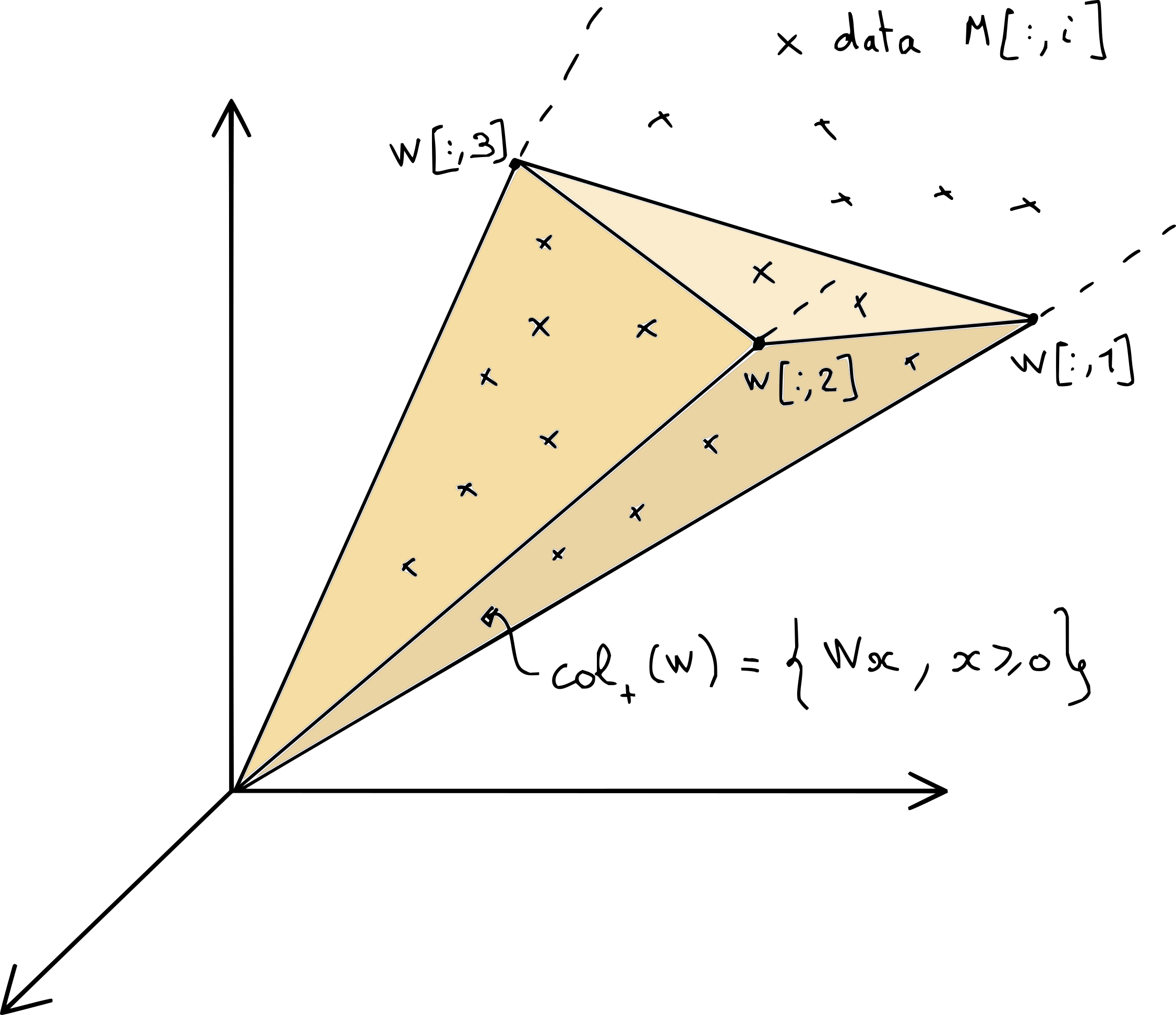
Fig. 9 A graphical illustration of one possible NMF of data matrix \(M\). The cone \(\cp{W}\) collects all the positive combinations of columns of matrix \(W\), and must contain all the columns of matrix \(M\).#
With this interpretation, it is simple to deduce the non-uniqueness, in general, of NMF. Consider the dimension two and rank-two case, \(n_1=r=2\), in Fig. 10. As soon as \(M[:,1]\) or \(M[:,2]\) is elementwise positive, the purple areas are non-trivial and there are infinitely many solutions. The only way NMF can be unique when \(n_1\) equals the rank is if \(W=I\) is the only solution (up to scaling and permutation and its columns), since \(M = IM\) is always a valid NMF in that case.
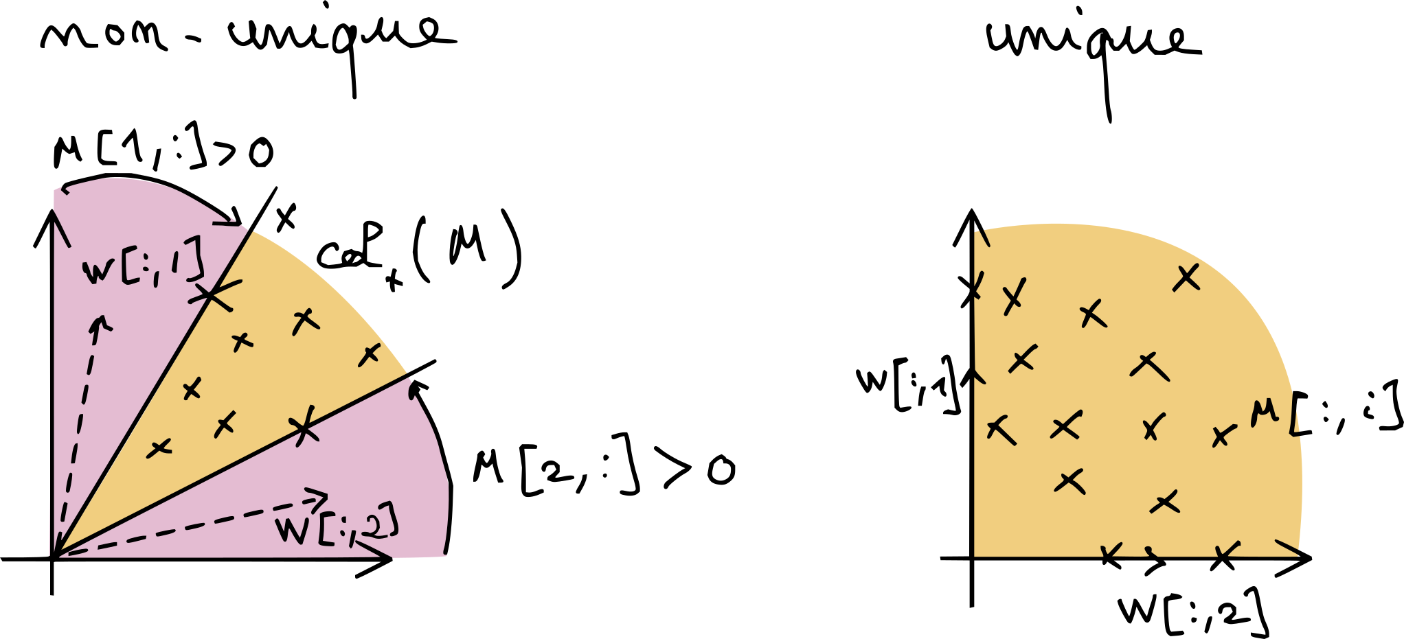
Fig. 10 A simple graphical explanation of why NMF without further regularization is generally non-unique. As long the purple areas around the cone spanned by the data points are sufficiently large, there may be infinitely many positive cones that contain the data. The situation is more complex in higher dimensions.#
A slightly more involved geometric representation of exact NMF can be obtained by projecting the data and model onto the unit simplex. The data then lives in the intersection of the nonnegative orthant and the unit simplex, which is a polytope.
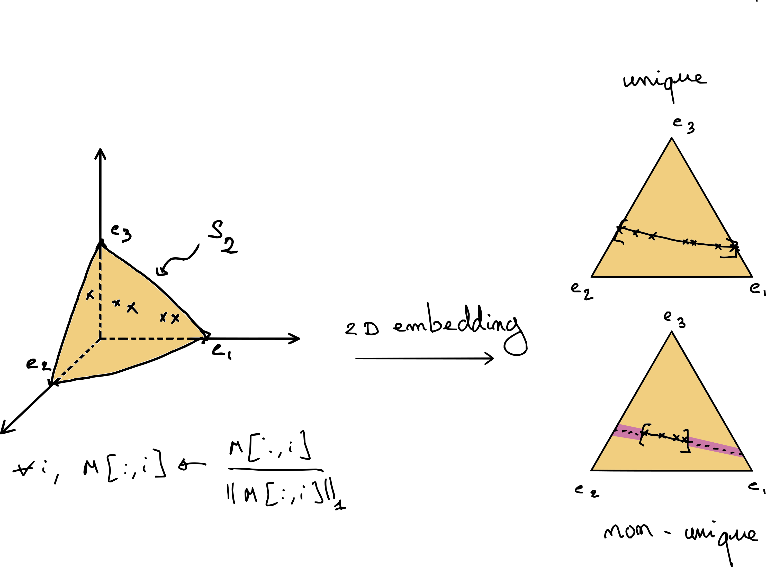
Fig. 11 Exact NMF in dimension 3 and rank 2. The data, after \(\ell_1\) normalization, lies on the simplex \(\mathcal{S}_2\). This embedding allows to visualize NMF in dimension three in the 2D plane. The right-hand side shows two possible scenarios, where NMF is either unique if the data points touch the border of the simplex, or not unique if the data are located on a segment strictly contained in the simplex.#
This geometric view allows for a finer description of identifiability in low-dimensional settings. Consider the case \(n_1=3\) and \(r=2\) in Fig. 11. We see that identifiability can be achieved without further regularization only if the data points touch the boundary of the simplex.
A key concept for NMF identifiability: sufficiently scattered
One of the many interesting results regarding NMF identifiability states that NMF is identifiable when both columns of \(H^T\) and \(W^T\) are sufficiently scattered inside the simplex. The book written by Gillis [Gillis, 2020] describes this technical condition in great detail. Intuitively, the sufficiently scattered condition for matrix \(H^T\) states that the columns of the data matrix \(X\), when looked from the inside of the cone spanned by matrix \(W\), touch the border of that cone and are sufficiently close to the extreme rays. A different interpretation is that the volume of the convex hull of columns of \(H^T\) is large enough to contain the largest sphere contained in the simplex (in fact, a little more is required). This explains the intuition behind sparse NMF and minimum- and maximum-volume NMF, discussed shortly below.
Regularized NMF#
Given the above observations, it is reasonable to assume in practice that NMF may not be unique. As with other LRA models, regularizations can be added to the model to remove unrealistic solutions.
There exist at least three main choices for regularizing NMF. First, one may assume that the columns of \(W\) are contained in the columns of the data \(M\). The resulting model, called separable NMF, writes
where \(\mathcal{K}\) is a subset of \(r\) indices in \([1,n_2]\). Separable NMF allows for restricting the set of NMF solutions drastically, since there is only a combinatorial number of column combinations. Separable NMF is interesting both for interpretability and algorithm design. A typical example is separable exact NMF in the rank-two case, which is solved in closed form using a simple algorithm that picks the largest vector in the data and then the vector farthest from that first component; see Fig. 12. Exact separable NMF in general can be solved in polynomial time with a variant of the QR with pivoting algorithm [Gillis, 2014, Gillis and Vavasis, 2014]. Separable NMF is incredibly useful in practice for initializing any NMF algorithm, since it is fast to compute. Because the templates \(W\) are extracted directly from the data, separable NMF often yields interpretable results that summarize key patterns in the data. Separable NMF, however, fails when the dataset contains no pure data points, which may occur when all data points are the result of non-trivial mixtures of several components.
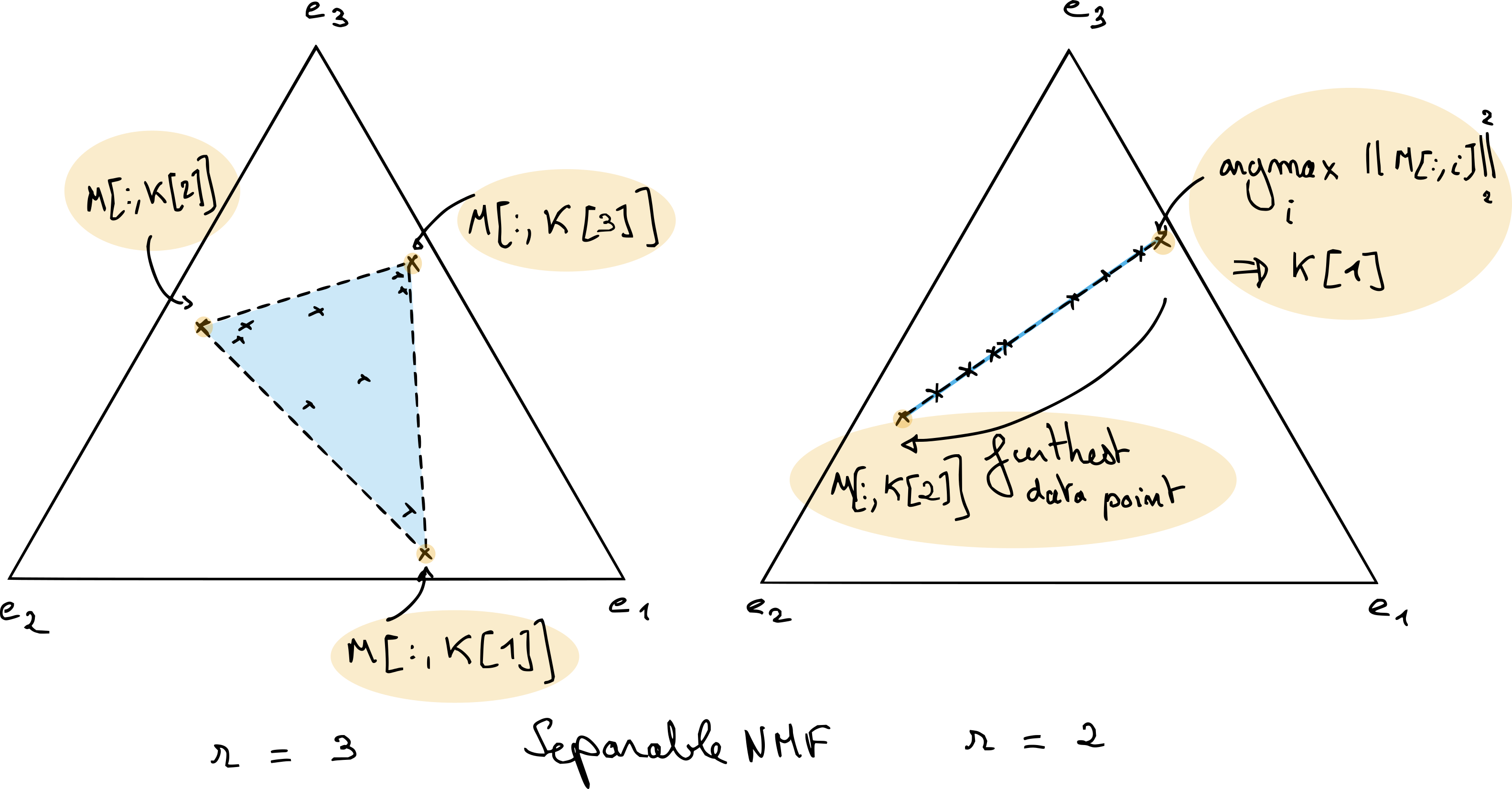
Fig. 12 Separable NMF finds the matrix \(W\) in the columns of the data matrix \(M\). In the particular case of rank-two separable NMF (on the right), the solution can be obtained by picking for the first columns of matrix \(W\) the data point with largest \(\ell_2\) norm after \(\ell_1\) normalization, and then choosing the furthest data point as the second column. When the rank is larger, algorithms exist that can compute exactly separable NMF in polynomial time, such as the Successive Nonnegative Projection Algorithm (SNPA) [Gillis, 2014]; the underlying idea behind SNPA is similar to that of OMP.#
A second variant of NMF is sparse NMF, in which the entries of the matrices \(W\) and/or \(H\) are pushed towards zero. A typical formulation of sparse NMF with \(\ell_1\) regularization writes
with \(\lambda\) a positive hyperparameter, that promotes sparsity in matrix \(H\) when large enough. Such regularized low-rank models are discussed further in Implicit regularization in rLRA. Sparse NMF can be unique when NMF is not, since sparsity pushes columns of matrix \(H\) towards the border of the simplex, maximizing volume.
A third regularized NMF model is the minimum-volume (or maximum-volume [Thanh and Gillis, 2026]) NMF. The idea behind minimal-volume NMF is to choose the matrix \(W\) to be as close as possible to the convex hull of the data. In a sense, it is a relaxation of the separability assumption that can still work when pure data do not exist. The minimization of the volume of the cone spanned by the matrix \(W\) can be related to the maximization of the volume of the columns of matrix \(H^T\). The volume of the columns of \(W\) can be measured as \(\log\det(W^TW)\), which is a concave function.
In many practical uses of NMF, it is important to consider whether regularized NMF should be considered instead. After working for several years with NMF on various applications, I believe many authors have underestimated the identifiability problem of NMF. A typical example is automatic transcription, where NMF has been used over the last two decades without, to the best of my knowledge, a proper discussion on the uniqueness of the results.
Fitting NMF#
To fit NMF to a dataset, several Python libraries are available. Scikit-learn has a nice implementation of both MU and cyclic coordinate descent, which allow for sparsity-inducing regularization. Nimfa is a toolbox dedicated to NMF that implements many variants of NMF, including Bayesian and graph-regularized NMF. It has not been updated since 2019, and as far as I know, it is geared towards flexibility rather than performance.
A third and probably less advertised option is to use nonnegative tensor decomposition available in tensorly. The interface is rather simple and, like in Scikit-learn, two algorithms are proposed, namely MU and alternating HALS. tensorly, in fact, implements HALS as a NNLS solver, which can be handy as a building block for other nonnegative factorization problems. Since I am a co-developer of tensorly, let us demonstrate how to perform a toy NMF factorization with tensorly.
import numpy as np
from tensorly.decomposition import non_negative_parafac_hals
import matplotlib.pyplot as plt

# Dimensions
n1, n2 = [3,50]
rank = 2

# Seed
rng = np.random.default_rng(5)

# Generating a dummy nonnegative matrix with exact NMF
W_true = rng.random((n1, rank))
H_true = rng.random((n2, rank))
M = W_true@H_true.T

# Computing NMF
out = non_negative_parafac_hals(M, rank, init="svd", n_iter_max=100, tol=0)
We = out[1][0]
He = out[1][1]
Me = We@He.T

# Computing final error
print(f"Final mean reconstruction error: {np.linalg.norm(M-Me)/n1/n2}")

# Plotting the 3d data points, true W positions as triangles and estimated W positions
# a. normalization of data, data_e and W
We = We / np.sum(We, axis=0)
W_true = W_true / np.sum(W_true, axis=0)
M = M / np.sum(M, axis=0)
Me = Me / np.sum(Me, axis=0)

# b. 3d plotting
fig = plt.figure(figsize=(12,10))
ax = fig.add_subplot(projection='3d', elev=20, azim=10)
# 3d data
for i in range(n2):
    ax.scatter(M[0,i], M[1,i], M[2,i], c='blue', label='Data points' if i==0 else "")
# increase markersize for better visibility
ax.scatter(W_true[0,:], W_true[1,:], W_true[2,:], s=100, c='red', marker='^', label='True W')
ax.scatter(We[0,:], We[1,:], We[2,:], s=100, c='green', marker='x', label='Estimated W')
ax.set_xlabel('Dimension 1')
ax.set_ylabel('Dimension 2')
ax.set_zlabel('Dimension 3')
plt.title('NMF: True vs Estimated W')
plt.legend()
plt.grid()
plt.show()
Final mean reconstruction error: 1.2146666877441276e-05
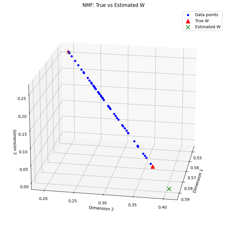
We can observe that the data matrix indeed follows an exact rank-two NMF, since all data points lie on a segment in the nonnegative orthant. Note that the true NMF with columns of matrix \(W\) close to the data points is not recovered by our NMF algorithm despite the small fitting error. Here, separable NMF or minimum-volume NMF would allow us to recover almost exactly the ground truth. An implementation of the nonnegative variant of QR with pivoting for NMF, SNPA [Gillis, 2014], is provided with this manuscript. Indeed, separable NMF in this toy example can recover a better estimation of the true parameter matrix \(W\), and therefore more accurate coefficients \(H\).
from tensorly_hdr.sep_nmf import snpa

_, We_snpa, He_snpa = snpa(Me, rank)
He_snpa = He_snpa.T
Me_snpa = We_snpa@He_snpa.T
print(f"Final mean reconstruction error with SNPA, {np.linalg.norm(M-Me_snpa)/n1/n2}")

# Plotting the 3d data points, true W positions as triangles and estimated W positions with SNPA
fig = plt.figure(figsize=(12,10))
ax = fig.add_subplot(projection='3d', elev=20, azim=10)
# 3d data
for i in range(n2):
    ax.scatter(M[0,i], M[1,i], M[2,i], c='blue', label='Data points' if i==0 else "")
# increase markersize for better visibility
ax.scatter(W_true[0,:], W_true[1,:], W_true[2,:], s=100, c='red', marker='^', label='True W')
ax.scatter(We[0,:], We[1,:], We[2,:], s=200, c='green', marker='x', label='Estimated W with NMF')
ax.scatter(We_snpa[0,:], We_snpa[1,:], We_snpa[2,:], s=150, c='magenta', marker='x', label='Estimated W with SNPA')
ax.set_xlabel('Dimension 1')
ax.set_ylabel('Dimension 2')
ax.set_zlabel('Dimension 3')
plt.title('NMF with SNPA: True vs Estimated W')
plt.legend()
plt.grid()
Final mean reconstruction error with SNPA, 1.974386306482247e-05
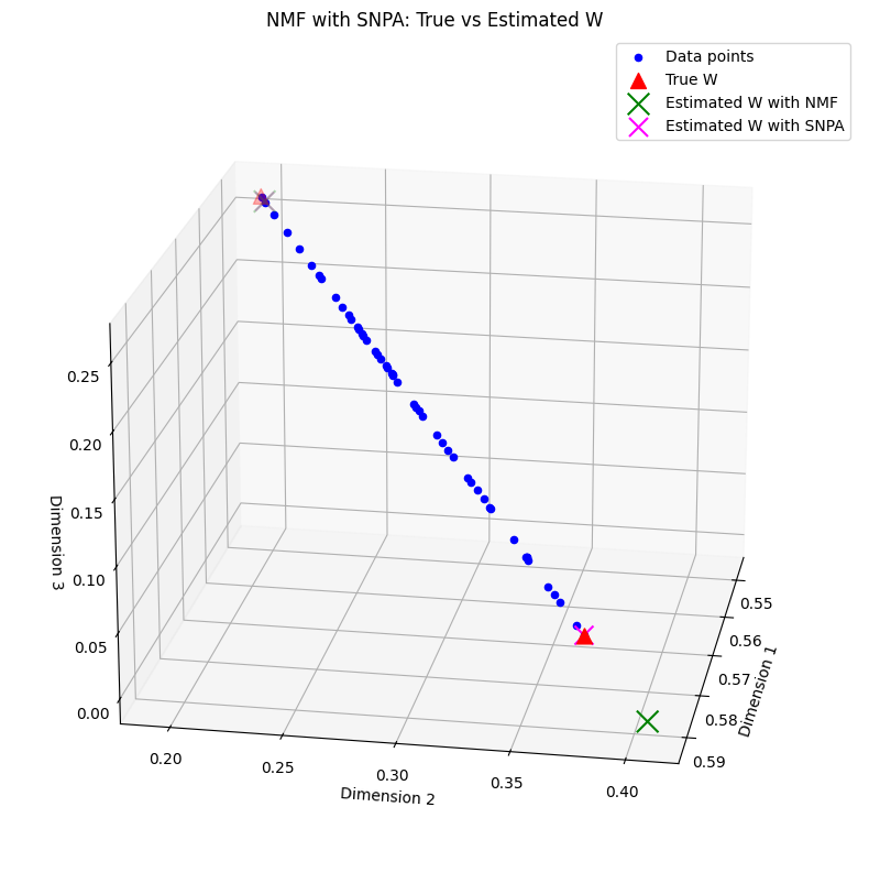
Note that in the rank-two case, exact separable NMF can be instead computed exactly with a cheaper algorithm. The simulation above is merely a toy example, and SNPA is useful for all separable NMF problems with rank greater than two.
Tensor decompositions#
Tensors are often loosely defined as multiway arrays, that is, extensions of matrices with more than two dimensions. In reality, there are several definitions of tensors in the world of applied mathematics that coincide:
Tensors can be seen as multiway arrays.
Tensors can be seen as representations of multilinear forms (like matrices represent bilinear forms).
Tensors can be seen as representations of multilinear maps (like matrices encode linear operators). The notion of covariant/contravariant spaces is defined in this context.
Tensors are vectors in a tensor space (like a matrix \(M\) equals \(\sum_{i,j} M[i,j]e_i e_j^T\) with \(e_i\), \(e_j\) canonical basis vectors), which is how I like to define them.
While for matrices, the coexistence of these concepts does not seem to pose significant issues in the scientific community, these definitions, while compatible, lead to serious misunderstandings between researchers of different scientific fields. In classical mechanics, tensors are generally regarded as multilinear maps, whereas in quantum mechanics, they are elements of tensor spaces of high order (one vector space per quantum particle in the system). In data science, they are generally considered multiway arrays, and in statistics, they are often used to describe higher-order moments. In algebra, tensors are used to represent higher-order polynomials and their associated multilinear form. This leads to confusing discussions, especially regarding the basis of representation for tensors, which is critical in the operator representation point of view but largely irrelevant in the multiway array point of view. These different views even gave birth to a dedicated Wikipedia page that clarifies these various definitions.
In these fields, tensors are used for different reasons, have different characteristics, and represent data and operators. My personal advice to fellow researchers, when faced with scary tensor concepts and notation, is to go back to the matrix case that most of us are more familiar with and then extrapolate the concepts from matrices to tensors. Some authors have long advocated that tensors are a completely different object from matrices, and that their study requires specialized tools and mathematical intuition. While this statement is not false, in my opinion, it is in fact largely exaggerated. What is special is not often tensors but rather unconstrained LRA for matrices and the existence of SVD and the Eckart-Young theorem. Most problems encountered when working with NMF, such as identifiability, nonconvex optimization, or NP-hardness, hold for many tensor decompositions, both constrained and unconstrained. A particularity of tensors, however, is the necessity of efficient high-order contractions, that is, computing sums of multiway arrays across many indices as fast as possible; see, for instance, this Dagstuhl report to which I modestly contributed [Bientinesi et al., 2022].
In the following, a minimal description of tensor decomposition is provided to understand the contributions summarized later in the manuscript. For a better reference on tensor decompositions, I advise reading either the recent book of Ballard and Kolda [Ballard and Kolda, 2025] for a quick practical understanding, or the book of Hackbush [Hackbusch, 2012] for a deep mathematical description of tensors. I also enjoyed reading an older reference from Laurent Schwartz [Schwartz, 1975] on tensor products.
Tensors and the tensor product#
The tensor product#
We start by defining a tensor space in terms of linear algebra. Tensor spaces emerge as a way to provide a “nice” vector space for bilinear objects. Consider the couple \((x,y)\in E\times F\) with \(E\) and \(F\) two given real (or complex) vector spaces. The carthesian product \(E\times F\) is a vector space of dimension \(\text{dim}(E) + \text{dim}(F)\), and scalar multiplication with a scalar \(\lambda\) write \(\lambda(x,y) = (\lambda x, \lambda y)\). The Cartesian product simply juxtaposes the vector spaces \(E\) and \(F\), but it does not allow much interaction between them. Notice, for instance, that there is no principled way in the Cartesian product to multiply each vector \(x\) and \(y\) by two different scalars. Vectors \(x\) and \(y\) in a Cartesian product are essentially living in two unrelated spaces.
In data mining and low-rank approximations in particular, there is a clear interest in extracting patterns that span across the two dimensions of a matrix. Think how NMF extracts patterns (column of matrix \(W\)) for each dimension jointly with the activations (columns of matrix \(H\)). Therefore, we need an underlying vector space that contains interactions between the two vector spaces, larger than the Cartesian product. One way to do this is to consider multilinear maps, such as the scalar product,
where \(u\) is a multilinear map acting on the couple \((x,y)\). The core idea of tensor spaces and the tensor product is to find a canonical way to map the couple \((x,y)\) to a vector \(\otimes(x,y):= x\otimes y\), where \(\otimes\) is the tensor product, such that the multilinear map \(u\) decomposes as a linear map \(w_u\) acting on the tensor product:
The tensor product is, therefore, a canonical multilinear map that can be used to make all multilinear maps linear. An important mathematical result, proved for instance in [Schwartz, 1975] and called the universality theorem, is that this canonical multilinear map \(\otimes\) always exists and that for any multilinear map \(u\) and fixed tensor product \(\otimes\), there is a unique linear map \(w_u\) such that \(u(x,y) = w_u(x\otimes y)\). The set \(E\otimes F:=\{x\otimes y, (x,y)\in E\times F\}\) is a vector space, coined the tensor product space. Its dimension is \(\text{dim}(E)\text{dim}(F)\) and it is generated by basis elements \(e_i\otimes f_j\) for two bases \(\{e_i\}_i\) and \(\{f_j\}_j\) of respectively vector spaces \(E\) and \(F\).
The tensor product itself is not unique. However, it can be shown that any two tensor products are related through an isomorphism. This fact is very well known to all data scientists. Take the outer product \(xy^T\), and the Kronecker product \(x\otimes_K y\). It turns out both are tensor products, related through a trivial isomorphism: row-first vectorization.
For most practical use cases, one may identify vector spaces \(E\) and \(F\) with \(\mathbb{R}^{n_1}\) and \(\R{n_2}\), and the tensor product with the outer product
Going back to the scalar product example, with the outer product as a tensor product, the linear map associated with the bilinear scalar product is the trace operator:
One interesting piece of multilinear algebra theory, however, is that, in finite dimensions, the vector space of linear maps acting on a tensor space is also a tensor space, of the form \(\mathcal{L}(E) \otimes \mathcal{L}(F)\) [Hackbusch, 2012]. The natural tensor product in linear operator spaces for matrix representation is the Kronecker product, and this can be used to generalize tensor decompositions to linear operators quite naturally, as done in the PhD thesis of Cassio Fraga Dantas [Dantas, 2019]. When considering linear operators acting on tensors, for instance \(A\) acting on \(x\) and \(B\) acting on \(y\), we simply write them in the form \((A\otimes B)(x\otimes y):= Ax\otimes By\).
Important
This discussion holds not only for two vector spaces \(E\) and \(F\), but for any number of vector spaces \(E_i\), with \(i\leq d\). A tensor is any element of the tensor space \(E_1\otimes \cdots \otimes E_d\); we call the integer \(d\) the order of the tensor, or the number of modes of the tensor. Mode \(i\), or dimension \(i\), denotes the particular vector space \(E_i\).
Rank-one tensors are generators of the full tensor space#
We have seen by construction that any vector \(x\otimes y\) for \((x,y)\in E\otimes F\) belongs to the tensor space \(E\otimes F\). Since \(E\otimes F\) is a vector space, we may add an arbitrary number of such vectors and stay inside \(E\otimes F\). This means that any vector of the form
with \(p\) some finite integer is in \(E\otimes F\). We call elements of \(E\otimes F\) of the form \(x\otimes y\) rank-one tensors.
This construction raises two immediate questions of crucial importance
Can all elements of \(E\otimes F\) be described as a sum of rank-one tensors? If so, how large must \(p\) be?
Are all elements of \(E\otimes F\) rank-one tensors, and if not, what is the smallest number of terms that describes a given tensor?
The answer to the first question is positive: rank-one tensors are generators of the linear space \(E\otimes F\). This is clear in finite dimension since for two bases \(\{e_i\}_i\) and \(\{f_j\}_j\) of respectively \(E\) and \(F\), the set \(\{ e_i\otimes f_j\}_{i,j}\) is a basis for \(E\otimes F\). With matrices and using the outer product, we are simply stating here that any matrix \(M\) can be written in the canonical basis
with \(e_i\) and \(f_j\) vectors null everywhere except in position respectively \(i\) and \(j\) where they contain one. This also shows that using more than \(d=\text{dim}(E)\text{dim}(F)\) is not required.
The answer to the second part of the second question is directly related to the canonical tensor decomposition described in the next section. Regarding the first half of the question, it is simple to exhibit a tensor that cannot be written as a rank-one tensor. Take \(e_1 f_1^T + e_2 f_2^T\) with the previous bases notations. If there exists a rank-one tensor \(xy^T\) such that \(xy^T = e_1f_1^T + e_2 f_2^T\), then denoting \(z_x\) an orthogonal vector to \(x\),
for the left-hand side, while
Because \(f_1\) and \(f_2\) are linearly independent, the two equalities cannot happen simultaneously, and therefore \(e_1 f_1^T + e_2 f_2^T\) cannot be written as a rank-one tensor (matrix). The counter-example holds for tensor spaces of higher order as well.
CP decomposition#
The Canonical Polyadic decomposition (CP decomposition or CPD), also called PARAFAC decomposition, is the decomposition of a given tensor into a sum of rank-one tensors with as few terms as possible [Carroll and Chang, 1970, Harshman, 1970, Hitchcock, 1927]. This minimal number of terms is called the rank of a tensor, and is an extension of matrix rank. Indeed, matrix rank can be described, among all possible equivalent definitions, as
when \(E\) and \(F\) are real finite-dimensional vector spaces.
Notice that the sum \(\sum_{i\leq q} x_i\otimes y_i\) can be written in matrix format as \(M=XY^T\), where matrices \(X\) and \(Y\) contain vectors \(x_i\) and \(y_i\) stacked columnwise. In the matrix case, the CP decomposition is therefore simply an exact unconstrained LRA model. Matrix CP decomposition is never unique, and can be computed efficiently with the SVD. An approximate CP decomposition, defined as an approximate LRA model, is also easy to compute with the truncated SVD.
From numerical linear algebra and data science perspectives, the CP decomposition for tensors with more than two modes is fundamentally different: the CP decomposition for higher-order tensors is identifiable under mild assumptions, but its computation can be extremely challenging.
CP decomposition for third-order tensor and identifiability#
Let us now discuss the tensor CP decomposition for real multiway arrays, with the outer product \((x\otimes y\otimes z)[i,j,k] = x[i]y[j]z[k]\) as the tensor product. For a third-order tensor \(T\) in \(\R{n_1\times n_2\times n_3}\), the CP decomposition of \(T\) is a minimal decomposition
where matrices \(A\), \(B\), and \(C\) are sometimes called the factor matrices of the CP decomposition, and the rank \(r\) is as small as possible.
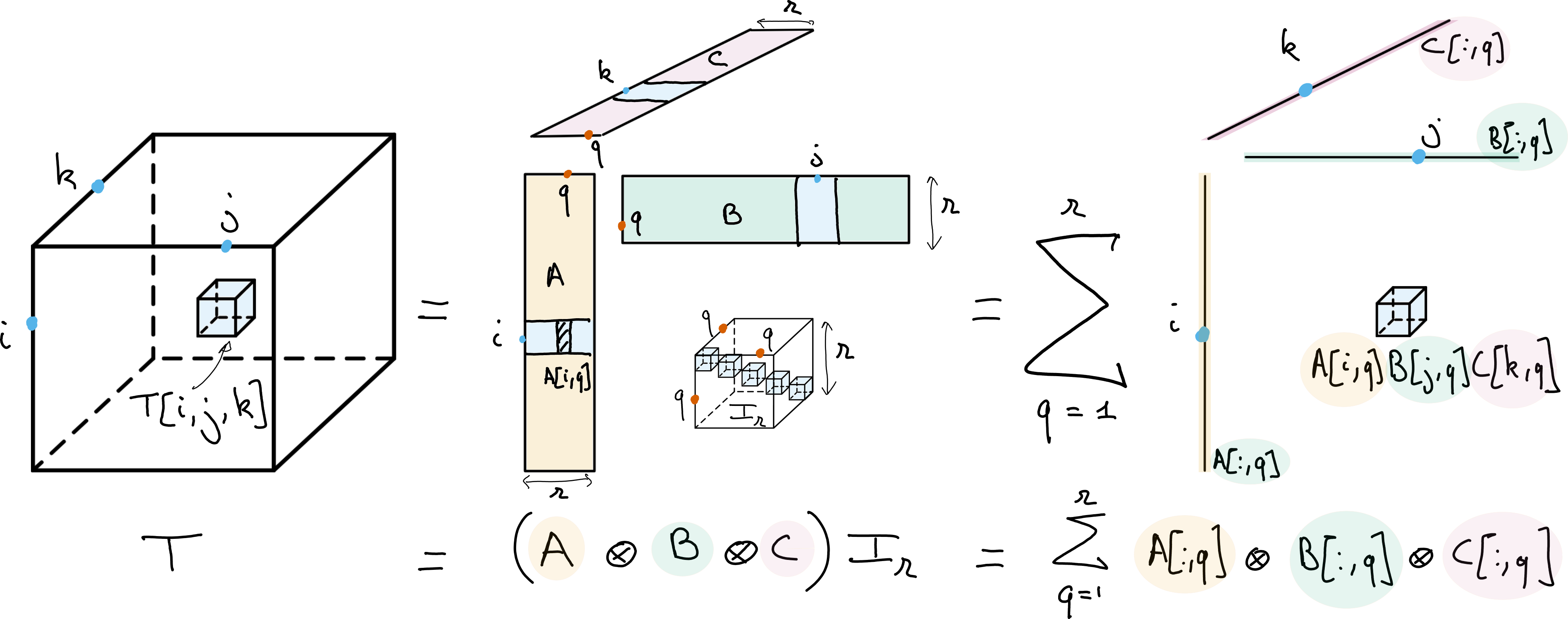
Fig. 13 Canonical Polyadic Decomposition (CPD) of rank \(r\) of a data tensor \(T\). The CPD can be viewed as a multilinear diagonalization technique, with bases \(A\), \(B\) and \(C\) respectively spanning the columns, rows and fibers of the tensor, or as an atomic decomposition into a sum of \(r\) rank-one tensors.#
The key property of the CP decomposition is that there is typically a unique set of rank-one tensors \(A[:,q]\otimes B[:,q] \otimes C[:,q]\) that decomposes a given tensor \(T\). If these factors can be computed numerically with guaranteed stability [Vannieuwenhoven, 2017] and if the CP decomposition matches a physically meaningful model, then the estimated factor matrices can be interpreted without the need for further regularization. This nice property can be contrasted with the matrix case, where regularizations, such as nonnegativity for NMF, are required to hope for identifiability. The most well-known identifiability conditions for the CP decomposition are probably the Kruskal condition; see, for instance, the accessible proof provided by Stegeman and Sidiropoulos [Stegeman and Sidiropoulos, 2007].
Why is CP decomposition identifiable while matrix LRA is not
When the CP decomposition was studied by Richard Harshman in psychometrics in 1970 [Harshman, 1970], he provided a simple proof from Jenrich of its parameter identifiability, albeit with strong assumptions. He had a very strong intuition for why the model could be identifiable. The core idea is that CP decomposition fixes rotation ambiguities observed in matrix LRA.
To see this, observe that the CP decomposition of a third-order tensor can be written in terms of coupled matrix factorization as
In other words, the CP decomposition is the joint diagonalization of each slice \(T[:,:,k]\) of the tensor. Joint diagonalization means that the same bases for the column and row spaces \(A\) and \(B\) are used for all slices.
To explain further why joint diagonalization fixes rotation ambiguities, let us assume that there are only two slices in the tensor, \(n_3=2\), and assume these two slices admit an exact CP decomposition with full rank matrices \(A\) and \(B\) and nonzero entries in one of the two columns of matrix \(C\). It is possible to estimate \(A\) and \(B\) directly from the tensor \(T\) using Jenrich’s algorithm. Observe that
which is exactly the nonzero part of the eigenvalue decomposition of the rank-deficient symmetric matrix \(T[:,:,1]T[:,:,2]^{\dagger}\). It is unique up to scaling and permutations, provided the singular values are distinct. Similarly, matrix \(B\) can be obtained from the eigenvalue decomposition of \(T[:,:,1]^{\dagger}T[:,:,2]\). The estimation of matrix \(C\) can be performed by solving an overdetermined linear system, with a unique solution since matrices \(A\) and \(B\) are full column rank.
Jenrinch’s algorithm shows that in many practical applications, the CP decomposition is essentially unique, even with two slices; while a low-rank factorization of each slice has infinitely many solutions, the intersection of these solution sets is singular, up to permutations and scaling ambiguities.
The CP decomposition model, like matrix LRA, has many applications. This is because multilinear maps are often encountered as simple yet efficient models in physics and mathematics for describing complex systems. The way tensor products are built on top of the multilinear tensor product ensures that the CP decomposition yields a sparse multilinear decomposition of the data. In other words, for each mode and for instance the first one, the map \(A\mapsto T\) is linear. The CP decomposition is essentially the description of a tensor as a sum of a few simple, discrete multilinear maps, the discrete analogue of a decomposition
The number of parameters in the CP decomposition is \((n_1+n_2+n_3)r\), much smaller than the \(n_1n_2n_3\) entries in the tensor \(T\) when the rank is smaller than the product of any two dimensions. Therefore, CP decomposition can also be used purely as a dimensionality reduction tool.
Note
There exist several shorthand notations for CP decomposition. Many authors use the so-called Kruskal notation \(T=\llbracket A, B, C \rrbracket\), which I will also use in this manuscript [Kolda and Bader, 2009]. However, in some settings, I prefer working with the more rigorous notation
where \(I_{r}[i,j,k] = \delta_{ir}\delta_{jr}\delta_{kr}\) is a diagonal tensor of ones. The tensor product \(\otimes\) is here meant in the sense of linear operators. This is in practice equivalent to the multiway product notation
but also makes explicit the tensor structure of the linear operators acting on tensors in finite dimensions.
Approximate CP decomposition computation#
On the surface, approximate CP decomposition is simply a particular case of approximate LRA. Let \(T\) be a data tensor to decompose. Approximate CP decomposition aims at finding a rank \(r\) tensor \(\llbracket A, B, C \rrbracket\) as close as possible to \(T\); the rank of the approximation \(r\) is fixed in advance. If the Frobenius norm \(\|T\|_F^2 = \sum_{i,j,k} T[i,j,k]^2\) is used as an error metric, the approximate CP decomposition computes the best rank-\(r\) approximation by solving the optimization problem
Like most LRA-related optimization problems, this is a nonconvex, multiblock optimization problem that can be addressed in practice by alternating optimization. The workhorse algorithm for fitting approximate CP decomposition is the Alternating Least Squares (ALS) algorithm. It updates each matrix \(A\), \(B\), and \(C\) in sequence, which, in general, can be done in closed form since the cost is quadratic in each parameter matrix. For instance, the update for the parameter matrix \(A\) is obtained by solving the linear system
where \(\odot\) is the Khatri-Rao product (columwise Kronecker products stacked horizontally), and \(\ast\) is the elementwise product. Matrix \(T_{[1]}\) is an unfolding of the tensor, namely, stacked slices of the tensor along the first mode. This formula can be obtained by computing the gradient of the cost with respect to the matrix \(A\) and then setting it to zero. ALS is a simple algorithm to describe at a high level, but, as is often the case in tensor computations, its efficient implementation requires advanced tools from numerical linear algebra and high-performance computing. There exist many other algorithms to compute approximate CP decomposition based on gradient descent (alternating or not), preconditioning, acceleration, algebraic methods, or second-order optimization [Acar et al., 2011, De Lathauwer et al., 2004, Rajih et al., 2008, Xu and Yin, 2013] (this list could be significantly longer; surveying this extensive literature is beyond the scope here).
Ill-posed approximation and nonnegative CP decomposition
Approximate CP decomposition is an ill-posed problem. The set of rank \(r\) tensors is not closed, therefore it may happen in theory that there exists no best rank \(r\) approximation [Hillar and Lim, 2013]. This causes practical issues that are difficult to predict and handle, such as slow convergence of ALS (so-called swamps) or even diverging components that cancel at infinity.
Since this manuscript is mostly concerned with regularized LRA, this problem is often avoided entirely. What is required to obtain the existence of a minimum in the approximation problem is coercivity of the cost on the domain definition. This is achieved when any coercive regularization is added, such as \(\ell_2\) regularization. The continuity of the cost, alongside coercivity, ensures that there exists a compact subset of the definition domain that contains the solution, which is therefore reached. In the context of CP decomposition, regularizations therefore not only help improve the interpretability of the parameters (although CP decomposition can be interpretable without such constraints, they often help in practice), but also make the approximation problem well-posed and easier to solve in terms of the optimization landscape.
A classic example of regularized CP decomposition is approximate nonnegative CP Decomposition (nCPD), defined as the solution to the optimization problem
Notice that the matrices have nonnegative entries. Algorithms to compute nCPD are similar to algorithms for solving NMF, and rely on NNLS solvers described extensively in Nonnegative regressions: NNLS and NNKL. A generic alternating algorithms that solves NNLS problems with respect to each factor matrix is sometimes called Alternating Nonnegative Least Squares (ANLS).
Notice also that coercivity is achieved with nonnegativity constraints, since the components cannot cancel out, and the cost function increases toward infinity as the components grow. Therefore, the best nonnegative low-rank approximation of a tensor always exists.
Tucker decomposition#
In the CP decomposition, the factor matrices \(A\), \(B\), and \(C\) can be seen as linear operators that map a diagonal tensor to the data tensor \(T\). In fact, using the linear operator tensor space point of view, the map \(A\otimes B\otimes C\) is a rank-one linear operator acting on tensors. The idea of Tucker decomposition is to generalize this observation by using rank-one linear operators to map large tensors to smaller tensors, thereby performing multilinear dimensionality reduction.
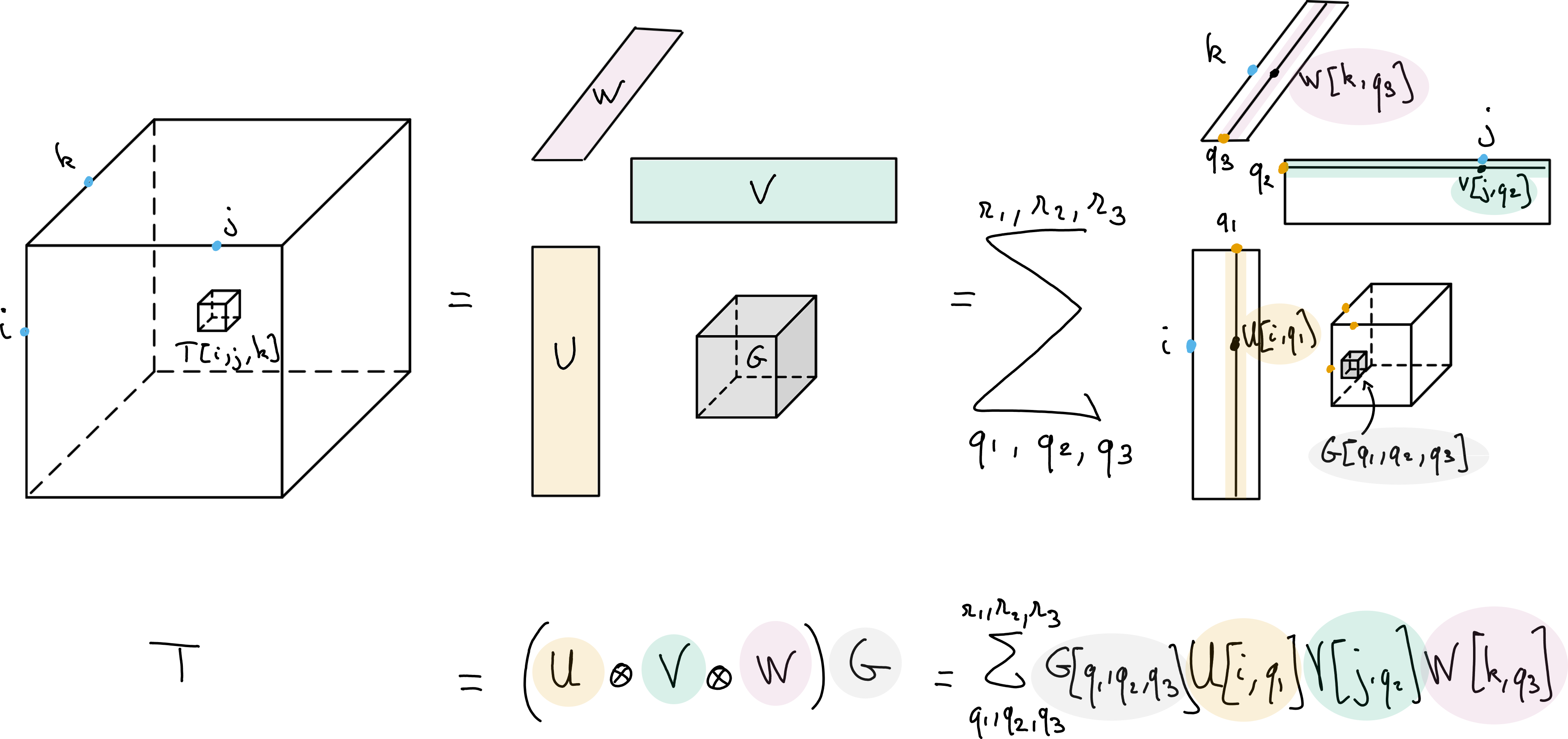
Fig. 14 Tucker decomposition of a data tensor \(T\), with multilinear ranks \(r_1\), \(r_2\) and \(r_3\). The Tucker decomposition can be viewed as a multilinear dimensionality reduction technique, with orthogonal bases \(U\), \(V\) and \(W\) respectively spanning the columns, rows and fibers of the tensor. Tensor \(G\) stores the coefficients into a tensor of size \(r_1\times r_2\times r_3\).#
For a data tensor \(T\in\R{n_1\times n_2\times n_3}\), the Tucker decomposition finds three matrices \(U\in\R{n_1\times r_1}\), \(V\in\R{n_2\times r_2}\), \(W\in\R{n_3\times r_3}\) and a smaller core tensor \(G\in \R{r_1\times r_2\times r_3}\) with \(r_i\leq n_i\) such that
with \(\times_i\) the multiway product defined above. Matrices \(U\), \(V\), and \(W\) as well as the core tensor \(G\) are the parameters of the model, which involves \(n_1r_1 + n_2r_2+ n_3r_3 + r_1r_2r_3\) parameters. This is significantly smaller than the number of entries in the tensor \(T\) when the so-called multilinear ranks \(r_i\) are smaller than the tensor dimensions. A tensor following an exact Tucker decomposition is written as
The Tucker decomposition is more similar to matrix LRA than the CP decomposition in terms of algorithmic development and uniqueness properties. Tucker decomposition has rotation ambiguities in each mode, since \(U\times_1 G = (UQ\times_1) (Q^T\times_1G)\) and is therefore never unique without further regularizations. Orthogonality is typically employed on each mode [Lathauwer et al., 2000], although nonnegativity is also a popular choice [Cohen et al., 2017, Mørup et al., 2008] that I have worked with, see Summary of HDR contents. The identifiability of Nonnegative Tucker decomposition is a longstanding problem that has seen some recent progress [Saha et al., 2025].
Tucker decomposition with orthogonality constraints can be computed almost exactly with the HOSVD algorithm [De Lathauwer and Vandewalle, 2004].
Tucker decomposition vs Tucker format
Because the Tucker decomposition lacks identifiability, it is more often used as a means of dimensionality reduction. In some computer science and applied mathematics communities, it is therefore called the Tucker format, while decomposition is used for models with uniqueness properties. I agree with this observation, but still refer to the Tucker format as the Tucker decomposition in this manuscript, as it is more common in the data science community.