
Nonnegative regressions: NNLS and NNKL#
Note
This section is based partly on a doctoral course I taught at the doctoral school of ITWIST 2020, and partly on more recent works around the MU algorithm. It is quite dense and long; however, nonnegative optimization problems are crucial tools to understand the rest of this manuscript.
Nonnegative regression problems are central in nonnegative low-rank approximations. Many LRA algorithms are based on alternating optimization, and optimization methods for nonnegative LRA are often heavily inspired by algorithms designed for nonnegative regression. Nonnegative regression is a class of optimization problems defined as
where \(f(y,z)\) is a nonnegative, separable, convex (with respect to the second variable) loss function comparing two vectors \(y\in\mathbb{R}^{m}\) and \(z\in\mathbb{R}^{m}\) elementwise, and \(W\in\mathbb{R}^{m\times n}\) is an observation matrix. The constraint \(x\geq 0\) is meant elementwise. Typically, both the observations \(y\) and the matrix \(W\) are also elementwise nonnegative. This section introduces two particular nonnegative regression problems, Nonnegative Least Squares (NNLS) and Nonnegative Kullback-Leibler regression (NNKL), that will be of particular interest for the rest of the manuscript.
Nonnegative Least Squares#
NNLS is a classic quadratic optimization problem, maybe one of the simplest generalizations of ordinary least squares. I am unsure of its origin, but the oldest mention of NNLS I am aware of is in the book of Lawson and Hanson on optimization methods for least squares problems [Lawson and Hanson, 1974]. Unlike ordinary least squares, however, NNLS does not have, in general, a closed-form solution.
Problem description#
NNLS can be formulated as the following optimization problem, with \( f\left(y,Wx\right)= \|y - Wx\|_2^2\):
In general, the projected unconstained least squares estimate, \(\left[W^{\dagger}y\right]^+\), is not a solution to NNLS, see Proco-ALS for fast nCPD for more details.
The cost function of NNLS is coercive (with respect to \(z\)) and continuous and the set of admissible solutions is non-empty, which ensures the existence of a solution. If matrix \(W\in\mathbb{R}^{m\times n}\) is full column rank, which is often the case in low-rank approximation problems, then the cost is also strongly convex (and Lipschitz-smooth), ensuring the NNLS solution is unique. When the matrix \(W\) is not full column rank, the discussion on the uniqueness is more difficult. One of the interests of NNLS over ordinary least squares, however, is that the solution for underdetermined systems can still be unique, see the NNLS KKT conditions below.
Geometric interpretation#
When \(W\) has desirable properties such as elementwise nonnegativity, NNLS is equivalent to the orthogonal projection of the input vector \(y\) on a pointed cone. Indeed, defining \(\cp{W} = \{Wx, x\geq 0\}\), we see that \(\cp{W}\) is always a cone. Let \(Wx_1,Wx_2\in \cp{W}\), for any nonnegative weights \(\lambda_1\) and \(\lambda_2\), it holds that \(\lambda_1 Wx_1 + \lambda_2Wx_2 = W (\lambda_1 x_1 + \lambda_2 x_2)\) is in \(\cp{W}\). NNLS finds the closest vector \(z\) to the input \(y\) in \(\cp{W}\),
which is exactly the orthogonal projection on \(\cp{W}\). Depending on the matrix \(W\), the cone \(\cp{W}\) can either be the whole search space \(\mathbb{R}^m\), or a pointed cone. The latter is the commonly encountered case in nonnegative LRA problems, in particular when the matrix \(W\) is elementwise nonnegative. Below is an illustration in dimensions \(m=n=3\).
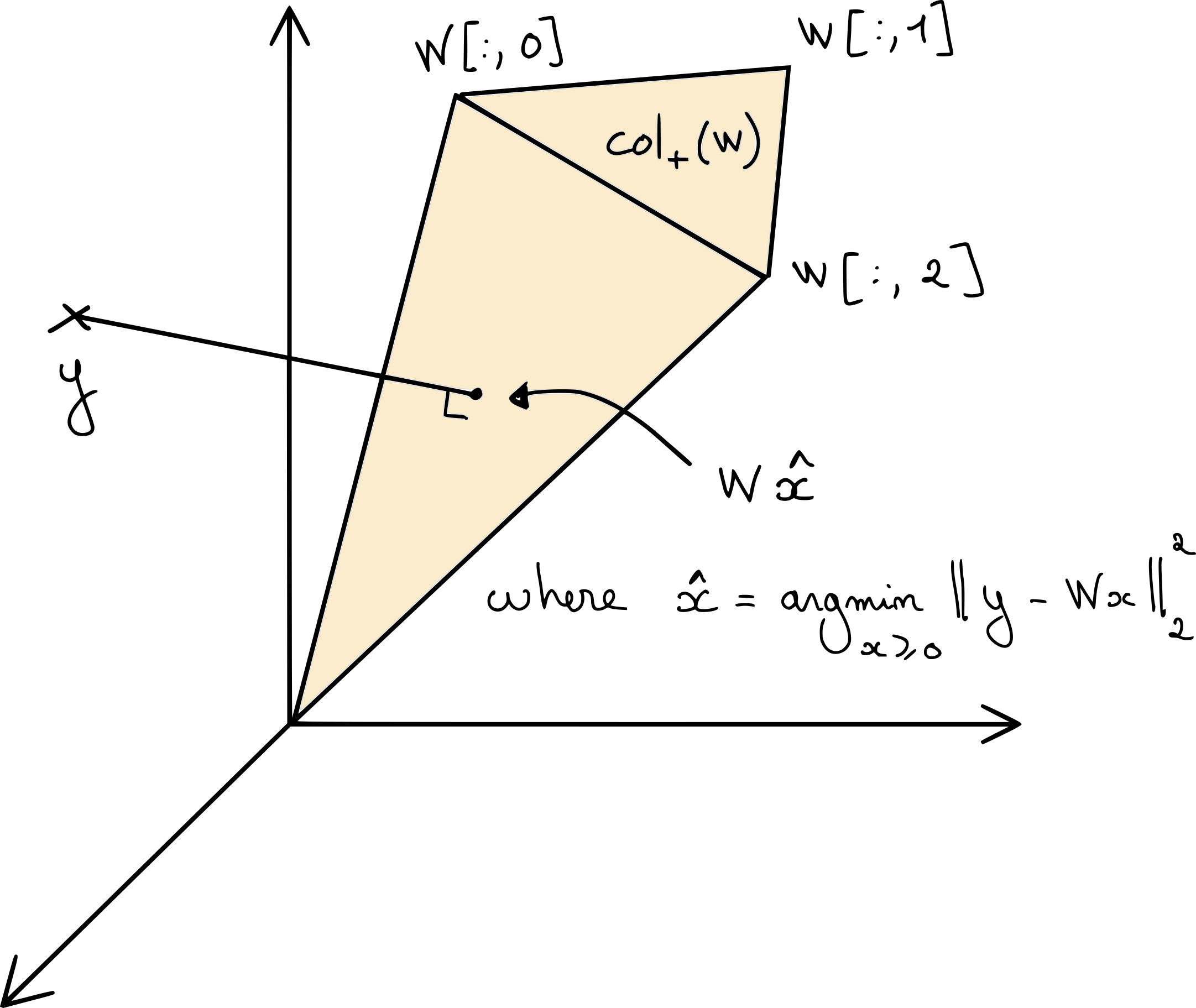
Fig. 15 A graphical illustration of the projection of data vector \(y\) on the cone \(\cp{W}\) collecting all the positive combinations of columns of matrix \(W\). The NNLS problem is equivalent to computing the coefficients of the projected data vector in the cone; note that when the data vector \(y\) is outside \(\cp{W}\), as illustrated here, the solution is sparse since the projection is located on a facet of the cone.#
From this geometric interpretation, we can deduce a few results:
If the measurement vector \(y\) lies inside the cone \(\cp{W}\), then an exact reconstruction is possible. We show with the KKT conditions that the least squares estimate \(W^{\dagger}y\) is a NNLS solution. The solution may be non-unique.
If matrix \(W\) has more columns than rows, but these columns are in general position, and vector \(y\) lies outside \(\cp{W}\), then in general the NNLS solution is unique.
When vector \(y\) lies outside the cone \(\cp{W}\), the projection solution \(z^\ast = Wx^\ast\) is located on a facet of the cone. In fact, it is the orthogonal projection of \(y\) on this facet. Hence, \(x^\ast\) may be sparse.
These results can be formalized using the KKT conditions.
KKT conditions and the night sky theorem#
Deriving the Karush-Kuhn-Tucker conditions (see, e.g., [Boyd and Vandenberghe, 2004]) for NNLS is not difficult, but very instructive. Denoting \(\lambda\geq 0\) the dual variable for the nonnegativity constraint, the Lagrangian writes
and the optimality conditions are:
Primal feasibility: \(x^\ast\geq 0\).
Dual feasibility: \(\lambda^\ast \geq 0\)
Complementary slackness: \(\lambda^\ast[i]x^\ast[i]=0\) for all \(i\leq n\).
Fermat rule: \( \nabla_x\mathcal{L}(x^\ast, \lambda^\ast)= 2W^T(Wx^\ast - y) - \lambda^\ast = 0\).
We can refine these conditions by introducing the support \(S^\ast\) of a solution; the support \(S(x)\) is the set of indices of the nonzero entries of the vector \(x\). The Fermat rule, combined with complementary slackness, then yields
with \(r = y - W[:,S^\ast]x[S^\ast]\) the residual of the projection of \(y\) on the cone \(\cp{W}\). When \(y\) is in the cone \(\cp{W}\), the residual \(r\) is null, and little can be said about the matrix \(W[:,S^\ast]\). However, when \(y\notin\cp{W}\), it must hold that \(r\neq 0\). Then any column \(W[:,i]\) of matrix \(W\) where \(i\in S^\ast\) is in the hyperplane \(r^⟂\) of dimension \(m-1\).
If there is no group of \(m\) columns of matrix \(W\) that are linearly dependent, that is, if \(\text{spark}(W)>m\), then there can be only a single subset of at most \(m-1\) linearly independent columns of matrix \(W\) in \(r^⟂\). This can happen even if matrix \(W\) has more columns than rows; we only require here that no subset of \(m\) columns is linearly dependent (and in particular cannot belong to \(r^\perp\)). With this observation, we can conclude that \(S^\ast\) has size at most \(m-1\), i.e., NNLS solutions, under some conditions, are generally sparse. Moreover, the Fermat rule gives \(x^\ast[S^\ast] = W[:, S^\ast]^\dagger y\): knowing the support of the solution is enough to find the solution itself (up to solving a linear system).
Theorem 2 (Night sky theorem [Byrne 1981])
Suppose \(y\notin \cp{W}\) and \(\text{spark}(W)>m\). Then the NNLS problem admits a unique solution which has at most \(m-1\) nonzeros.
The nice name for this result, which emphasizes the sparsity of NNLS solutions, was suggested to me by Cédric Herzet and Clément Elvira. While I am unsure of the name’s true origin, the result itself is proved in [Byrne, 1981]. The night sky theorem is useful to derive the active-set algorithm for NNLS.
Nonnegative Kullback-Leibler regression (NNKL)#
Sometimes, using the Euclidean norm to measure discrepancies between the measurement vector \(y\) and the model \(Wx\) is undesirable. There are at least two reasons why the Euclidean norm might be avoided:
Euclidean norm is sensitive to outliers. More generally, it penalizes large errors more than small errors. In applications such as music information retrieval, the data exhibit wide dynamic ranges, and small measurement values are as important as large ones.
From a statistical estimation point of view, the solution of NNLS is the Maximum Likelihood Estimator (MLE) of variable \(x\) when the noise model is Gaussian. For other noise models such as Poisson,
\[ y \sim \mathcal{P}\left(Wx\right), \]the MLE is obtained by the minimization of another cost function.
These two observations are connected: under the Poisson distribution, the larger the expected observation \(Wx,\) the larger the noise, but the variance also grows with \(Wx\). This means that small data values are more likely to be accurate than large values (in absolute value, not in relative error).
NNKL problem definition#
The MLE for Poisson noise implies the minimization of the KL-divergence between a measurement vector \(y\) and some vector \(z\in\mathbb{R}_+^{m}\), defined as the separable function
see below for the estimator derivation. The nonnegative regression problem with KL-divergence as a loss function, that is coined NNKL in this manuscript, is the optimization problem
where we have set \( f\left(y,Wx\right) = \sum_i \KL{y[i],W[i,:]x}\). Below are two interactive plots showing the graph of KL-divergence in 1D and 2D.
# Showing plots for 1d Kullback Leibler with slider for data position
x = np.linspace(1e-5, 10, 300)

def kl_divergence(p, q):
    """Calculate the KL divergence between two distributions."""
    return np.sum(p * np.log(p / q) + q - p)

y = np.zeros_like(x)
p = 2.5  # Initial reference distribution parameter
for i, q in enumerate(x):
    y[i] = kl_divergence(p, q)
# Data grid
xmax=10
ymax=10
x = np.linspace(1e-5, xmax, 400)
y = np.linspace(1e-5, ymax, 400)
X, Y = np.meshgrid(x, y)

# Initialize Z
Z = np.zeros_like(X)
ref_x, ref_y = 2.5, 2.5
for i in range(X.shape[0]):
    for j in range(X.shape[1]):
        q = np.array([X[i, j], Y[i, j]])
        p = np.array([ref_x, ref_y])
        Z[i, j] = kl_divergence(p, q)
Difficulties#
Compared to NNLS, which is a quadratic program, NNKL is, in general, significantly more difficult.
Smoothness issue#
Maybe the most commented-on difficulty for NNKL is the lack of Lipschitz-smoothness of the KL-divergence at zero. Lipschitz-smoothness is a crucial property in numerical optimization, used to derive descent conditions for first-order algorithms. In a nutshell, a function \(f\) which is twice differentiable over a convex set is \(l\)-Lipschitz-smooth if its Hessian can be bounded by \(lI\). This implies, using the second-order Taylor expansion and majorizing the second-order terms and remainder [Beck, 2017], that for any vector \(x\) and local perturbation \(z\) the following descent lemma holds:
Lipschitz-smoothness, therefore, ensures that globally, the slope of the function \(f\) does not change too fast. Combined with strong convexity arguments, Lipschitz continuity is the key ingredient for proving the convergence of the gradient descent algorithm with fixed stepsize. However, the second-order derivative of KL-divergence is \( \frac{\partial^2\KL{y,z}}{\partial z^2} = \frac{y}{z^2} \), which is unbounded near zero. Therefore, solving NNKL with first-order algorithms is challenging because no stepsize selection rule guarantees convergence. In practice, for sparse measurement vectors \(y\), the lack of Lipschitz-smoothness makes many out-of-the-box solvers inefficient for NNKL. Fig. 16 provides additional intuition.
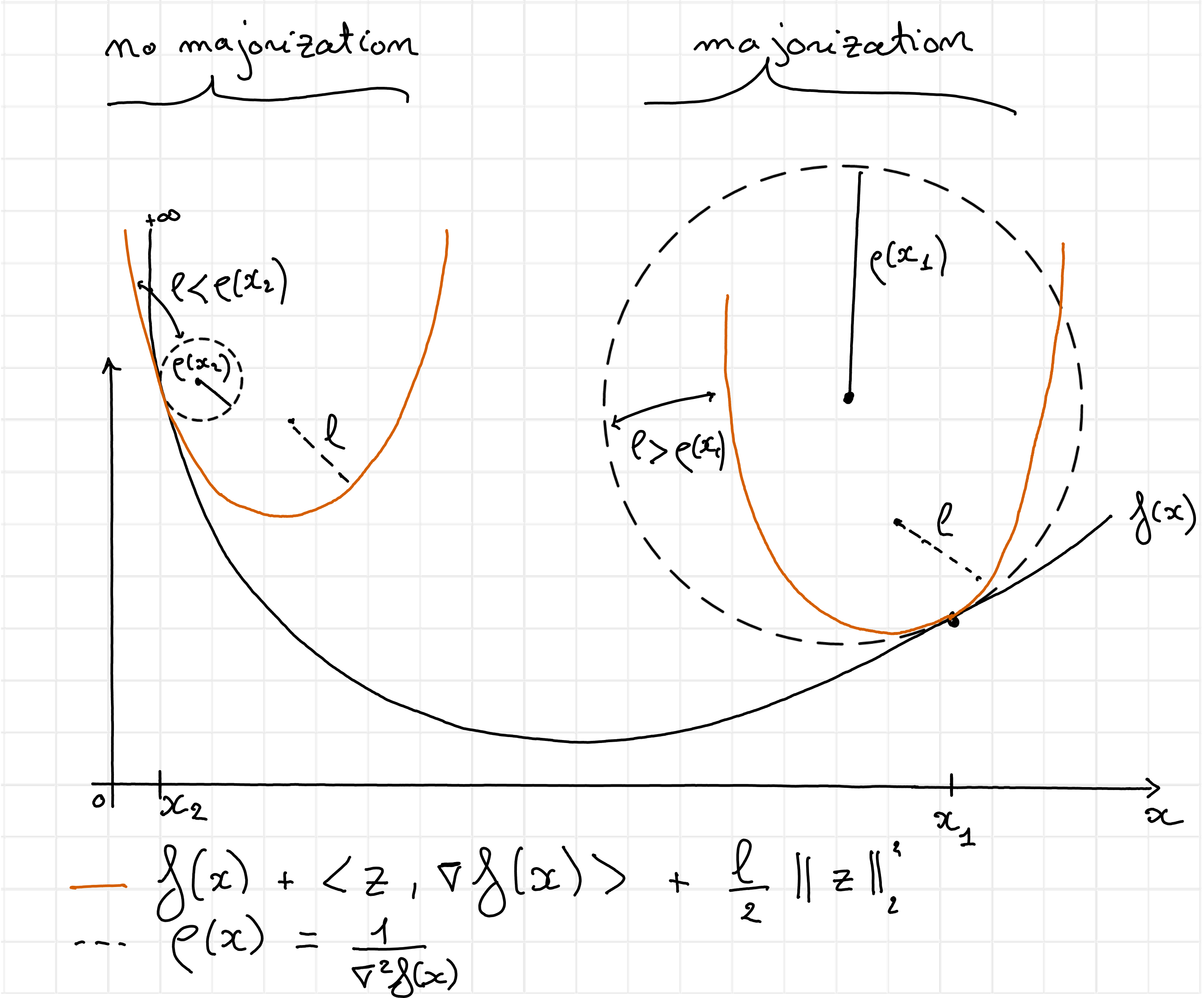
Fig. 16 A globally Lipschitz-smooth function can be bounded globally by a local quadratic approximation at any point with a fixed curvature \(l\). In this illustration, the curvature \(\rho(x)\) of the cost function \(f\) varies from flat (on the right) to steep (on the left). To ensure that a quadratic majorant can be defined everywhere with the same curvature \(l\), because to loss here diverges toward infinity near zero, the curvature must be chosen arbitrarily small. This is therefore an example of a function which is not Lipschitz-smooth. A direct consequence of this lack of smoothness is that it is impossible to define a constant stepsize for a gradient descent algorithm which guarantees that the cost decreases at each iteration. The gradient step, that computes the minimum of a quadratic majorant at each iteration, may reach a value below zero if initialized too far on the right (where the local curvature allows large stepsizes), while it will lead to exploding behavior near zero since the gradient of the cost is arbitrarily large. Gradient descent for KL-divergence is therefore typically employed with tiny stepsizes and strict positivity constraints that yield slow convergence.#
Convexity issue#
Another important issue with the KL-divergence is that, although it is strictly convex, it is not strongly convex. Indeed, the KL-divergence is asymptotically linear when \(z\) is much larger than \(y\). This causes problems in particular when the data measurement \(y\) is sparse or exhibits large dynamics. Strong convexity guarantees linear convergence rates for gradient descent; when the cost function is not strongly convex, first-order algorithms might converge sub-linearly [Beck, 2017]. In the extreme case where \(y\) has many zeros, a significant part of the cost is linear, and convex first-order optimization techniques are, in general, ill-suited for linear programming.
Smoothness and convexity issues combined imply that there may not exist a safe stepsize and a linear convergence rate for gradient descent applied to NNKL. In the following, we explore preconditionned first-order algorithms that partially avoid these issues.
Support issue#
A third, more subtle issue with NNKL, compared with NNLS, is that even if the support of the solution \(x^\ast\) is known, the solution cannot be computed in closed form. Indeed, the KKT conditions write
Primal feasibility: \(x^\ast\geq 0\).
Dual feasibility: \(\lambda^\ast \geq 0\)
Complementary slackness: \(\lambda^\ast[i]x^\ast[i]=0\) for all \(i\leq n\).
Fermat rule: \( \nabla_x\mathcal{L}(x^\ast, \lambda^\ast)= W^T(1 - \frac{y}{Wx^\ast}) - \lambda^\ast = 0\).
On the support \(S\) of the solution the slack variables \(\lambda\) are null, which yields
Unlike NNLS, to the best of my knowledge, this system cannot be solved in closed form in general. Interestingly, one may observe that the residual vector \(r = 1 - \frac{y}{Wx^\ast} \), uniquely defined because \(Wx^\ast\) is unique [Tibshirani, 2013], must be sparse. The argumentation is in fact similar to the proof of the night sky theorem: the residual \(r\) belongs to the null space of \(W[:,S]^T\); together with the spark condition on matrix \(W\), this implies that \(S\) is of size at most \(m-1\).
Another observation is that we can rewrite the Fermat rule on the solution support as
This rule is similar to the projection on the cone \(\cp{W}\) found in the KKT conditions for NNLS, with a preconditioning \(\text{diag}\left(Wx^\ast\right)^{-1}\). We may therefore interpret NNKL as a non-orthogonal projection on the cone \(\cp{W}\). If we further assume that \(Wx^\ast \approx y\) and \(y>0\), NNKL is approximately the projection of \(y\) on the preconditionned cone \(\cp{\text{diag}(y)^{-1}W}\). This point of view sheds light on why algorithms for solving NNKL often rely on a combination of preconditioning and first-order methods.
Optimal scaling#
A last but important observation on NNKL is that the solution \(Wx^\ast\) must satisfy a simple scaling condition. Indeed, consider the optimal scaling problem
Supposing the unconstrained solution can be positive, the Fermat rule from the KKT conditions gives
showing that an optimal solution \(x^\ast\) must satisfy \(\sum_{i,j} W[i,j]x[j] = \sum_{i} y[i]\). We find that \(\sum_{j} \left(\sum_{i}W[i,j]\right) x[j] = \sum_{i} y[i]\). By scaling the columns of matrix \(W\) to sum to one, we find that the marginals of \(x\) and \(y\) must match. Therefore, an algorithm that solves NNKL can be refined by scaling the initial and output estimates \(x\).
Note
If nonnegativity constraints are dropped and the observation matrix \(W\) is right-invertible, the linear system \(y=Wx\) has at least one exact solution, and the Euclidean norm or the KL-divergence minimization problems have a common solution \( x^\ast = W^\dagger y\). This observation emphasizes the importance of the nonnegativity constraints in NNLS and NNKL, which act as an informative prior. Solutions to NNLS and NNKL can be arbitrarily far from the right pseudo-inverse and its projection on the nonnegative orthant, see the end of Proco-ALS for fast nCPD for an illustration for NNLS.
Algorithms for NNLS and NNKL#
There is a vast literature on optimization algorithms for solving NNLS, NNKL, or both, some of which is included in later parts of this manuscript. Listing all these methods, with their advantages and disadvantages, is an important but tedious task to which I will devote time in the coming years; see the discussion on research perspectives. In the rest of this section, only the most useful NNLS and NNKL algorithms for the manuscript are introduced: Active-Set (AS), HALS, and MU.
Active-set (NNLS only)#
A workhorse algorithm to solve NNLS is the AS algorithm proposed by Lawson and Hanson in 1974 [Bro and De Jong, 1997, Lawson and Hanson, 1974]. It is based on the observation that, knowing the support of the solution \(S(x^\ast)\), the solution itself can be computed using the unconstrained least squares estimate restricted to this support. AS therefore iteratively searches for the support of the solution. It works similarly to the OMP algorithm [Pati et al., 1993], where a candidate index is first added to the current estimation of the solution support, and the unconstrained least squares estimate restricted to the current support estimate is then computed. However, unlike greedy sparse approximation algorithms, AS includes a third step that thins the support. Below is a pseudo-code for AS and a simple example. We then describe each step in more detail. We will see that any step taken by the AS algorithm has to decrease the cost function.
def get_support(x):
   # returns the support of input vector x
   return list(np.where(x>0)[0])

def get_neg_support(x):
   # returns the support of input vector x
   return list(np.where(x<0)[0])

def activeset(y,W,x):
   # Initialize the support and restricted LS solutions
   supp = get_support(x)
   res = y - W@x
   print(f"Residual: {np.linalg.norm(y - W@x)}, support {supp}")

   # main AS loop, stop when the support does not change
   iter = 0
   old_supp = [-1]  # anything different than initial support
   while supp != old_supp:
      iter += 1
      old_supp = copy(supp)
      print(f"Iteration {iter}")
      # 1. Support update: find the "most negative" Lagrange multiplier
      if len(supp) < len(x):  # if the support is full, do not update the support (only happens at init)
         dual_params = W.T@res
         dual_params[supp] = -np.inf # ignore entries corresponding to the current support
         idx = np.argmax(dual_params)
         bisect.insort(supp, idx)  # insert support index while keeping sorted

      # 2. Unconstrained Least Squares restricted to the support
      ls_sol = np.linalg.lstsq(W[:,supp], y, rcond=None)[0]
      # embed ls_sol into full space
      ls_sol_full = np.zeros_like(x)
      ls_sol_full[supp] = ls_sol
      neg_supp = get_neg_support(ls_sol_full)

      # 3. Support iterative refinement, to ensure ls_sol is nonnegative
      while len(neg_supp) > 0:
         # Move along the line from the previous to the current candidate estimate, until the cone is crossed
         t = np.min(x[neg_supp]/(x[neg_supp]-ls_sol_full[neg_supp]))
         # Update x to decrease the cost along the line (x, ls_sol_full-x), until the constraints are active
         x = x + t*(ls_sol_full - x)
         # Update the support (remove one element)
         supp = get_support(x)
         # 2. Recompute LS solution on the new support and count negative entries
         ls_sol = np.linalg.lstsq(W[:,supp], y, rcond=None)[0]
         ls_sol_full = np.zeros_like(x)
         ls_sol_full[supp] = ls_sol
         neg_supp = get_neg_support(ls_sol_full)
         print(f"Residual: {np.linalg.norm(y - W@x)}, support {supp}")

      # Update x with new nonnegative ls_sol
      x = ls_sol_full
      res = y - W@x

      # printing error for following AS progress
      print(f"Residual: {np.linalg.norm(res)}, support {supp}")

   return x, supp
Observe how in the following examples, the support grows and shrinks with AS iterations, and the NNLS cost decreases every time vector \(x\) is updated.
np.random.seed(2)
m=6
n=50
W = np.random.rand(m,n)
support = [0,2,4]
xtrue = np.zeros(n)
xtrue[support] = np.random.rand(3)
y = W@xtrue + 0.1*np.random.randn(m)
x0 = np.zeros(n)
#x0 = np.random.rand(n)  # also works
x_opt, est_support = activeset(y,W,x0)
print("Optimal x:", x_opt)
print(f"Optimality criterion on estimated support: {np.linalg.norm(W[:,est_support].T@(y-W@x_opt))}")
print(f"Optimality criterion on true support: {np.linalg.norm(W[:,support].T@(y-W@x_opt))}")
Residual: 0.7332827438506135, support []
Iteration 1
Residual: 0.34036387671449636, support [np.int64(49)]
Iteration 2
Residual: 0.23756836129567335, support [np.int64(41), np.int64(49)]
Iteration 3
Residual: 0.16861002184543533, support [np.int64(7), np.int64(41), np.int64(49)]
Iteration 4
Residual: 0.15317817929560062, support [np.int64(3), np.int64(7), np.int64(41)]
Residual: 0.134132076527192, support [np.int64(3), np.int64(7), np.int64(41)]
Iteration 5
Residual: 0.10556301170510976, support [np.int64(3), np.int64(4), np.int64(7), np.int64(41)]
Iteration 6
Residual: 0.051953693458475836, support [np.int64(3), np.int64(4), np.int64(41), np.int64(44)]
Residual: 0.04449646221989812, support [np.int64(4), np.int64(41), np.int64(44)]
Residual: 0.04207535623520431, support [np.int64(4), np.int64(41), np.int64(44)]
Iteration 7
Residual: 0.04207535623520431, support [np.int64(4), np.int64(41), np.int64(44)]
Residual: 0.04207535623520431, support [np.int64(4), np.int64(41), np.int64(44)]
Optimal x: [0.         0.         0.         0.         0.00500251 0.
 0.         0.         0.         0.         0.         0.
 0.         0.         0.         0.         0.         0.
 0.         0.         0.         0.         0.         0.
 0.         0.         0.         0.         0.         0.
 0.         0.         0.         0.         0.         0.
 0.         0.         0.         0.         0.         0.25668643
 0.         0.         0.45111056 0.         0.         0.
 0.         0.        ]
Optimality criterion on estimated support: 1.8019635810009614e-16
Optimality criterion on true support: 0.004015649566386405
Initialization of AS#
Contrary to what is sometimes assumed, e.g., on the Wikipedia page on NNLS, the AS algorithm can be initialized with any nonnegative vector \(x\). If the initial guess is dense, the first step is skipped on the first iteration.
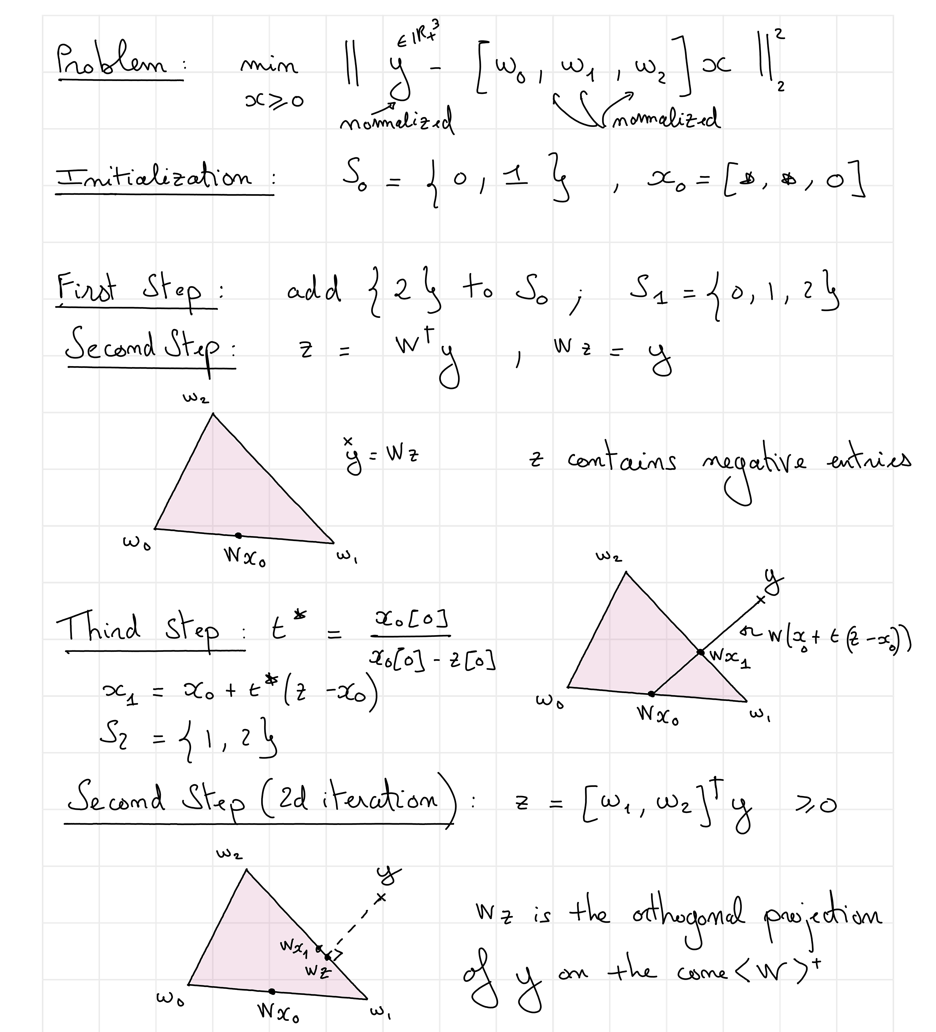
Fig. 17 An illustrated example of AS solving a three-dimensional NNLS problem.#
First step: selection#
Assuming the current support of \(x\) is not \([1,..,n]\), the selection step finds a “reasonable” index of an entry of \(x\) to add to the current estimation of the optimal support. A locally optimal choice is to select the index of the column of \(W\) most correlated with the residual \(r = y-Wx\) at the current iteration,
The local optimality is meant in the following sense: the scalar product \( \langle W[:,i], r\rangle \) is proportional to the orthogonal projection \(\Pi_{W[:,i]}(r)\) of the residual on the line spanned by vector \(W[:,i]\):
Another point of view is to observe that in the NNLS KKT conditions, the quantity \(W^Tr\) must be null on the optimal support and negative outside the support. Therefore, the selection step selects the largest nonzero scalar product and assumes it should be null. The last estimate of the residual is always an orthogonal projection on the span of \(W[:,S]\), hence no atom can be selected that is already in the support, or in the span of \(W[:,S]\), even without the explicit support constraint. This allows matrix \(W[:,S]\) to always be full column rank, except maybe at initialization.
This observation is also discussed in One-sparse dictionary-based LRA, but with \(\ell_2\)-normalized atoms.
Second step: restricted least squares regression#
The second step of AS is straightforward: one simply computes the unconstrained least squares estimate \(z = W[:,S]^\dagger y\), knowing that matrix \(W\) is full column rank. Note that at this step, the cost function can only decrease since the support increased in size due to the selection step. If \(z\) is nonnegative, we can safely continue the AS algorithm by looping back to step 1 with \(x=z\). However, if \(z\) is not an admissible solution, the AS algorithm enters a third step.
Third step: constraint satisfaction#
AS always ensures that the estimated \(x\) at the current iterate is admissible, and that the cost function decreases at each iteration. If \(z\) from step 2 is not admissible, the cost will have decreased, but it may be lower than the NNLS global solution. The main idea of AS is then to move the previous estimated \(x\) towards \(z\). This move will always decrease the cost because of the strong convexity of the map \(t\mapsto \|y - W[:,S](x+t(z-x))\|_2^2\). AS chooses the largest possible scalar \(t\) that ensures \(x+t(z-x)\) remains feasible, which is easily computed as
By updating \(x\) as \(x+t^\ast(z-x)\), at least one zero (and often, exactly one zero) is added in the current estimate \(x\). The cost has strictly decreased (unless \(t=0\), which can be shown to only happen at optimality), and the updated \(x\) is still admissible. The support needs, however, to be updated by removing all indices at which the interpolation reaches the cone boundary.
Then the algorithm loops back to step 2. An important remark is that for each support visited by AS, either the unconstrained least squares solution is admissible, and the current cost decreases, or the solution is not admissible and the support is updated while also decreasing the cost. Therefore, the same support can never be visited twice unless the algorithm has reached the global optimum. This shows that the AS algorithm terminates in a non-polynomial but finite number of steps: it can at most visit all the possible supports. When initialized close to the solution, AS can therefore be a very effective algorithm for solving NNLS.
HALS (NNLS only)#
The AS algorithm is the workhorse method for efficiently solving NNLS when the data are a one-dimensional vector. However, it is not well-suited for batch computations when solving the matrix NNLS problem of the form
Indeed, the AS algorithm would search for the optimal support of each column of the unknown matrix \(H^T\). These supports can all be different. The costly operation in AS is solving the least squares systems restricted to the current support estimate, and for matrix NNLS, these operations must be performed independently for each column. The fast AS algorithm [Bro and De Jong, 1997] improves on this issue by precomputing the grammians \(W^TW\) and \(W^TY\) in the case where \(W\) is a tall matrix.
For matrix NNLS, it is, however, useful to design an algorithm that can update all columns \(H^T[:,i]\) simultaneously. This is the rationale behind the HALS algorithm. HALS updates each row of matrix \(H\) sequentially, and this update is known in closed form. Indeed, notice that for any nonzero vector \(a\in\mathbb{R}^{m}\) and any matrix \(Z\in\mathbb{R}^{m\times n}\),
Indeed, this loss function is separable into \(n\) scalar problems
for any column index \(i\leq n\). The minimum of a scalar quadratic function under nonnegativity constraints is either the global minimum of the quadratic \(h[i] = \frac{w^TZ[:,i]}{\|w\|_2^2}\), or, if the global minimiser is negative, zero, see Fig. 18.
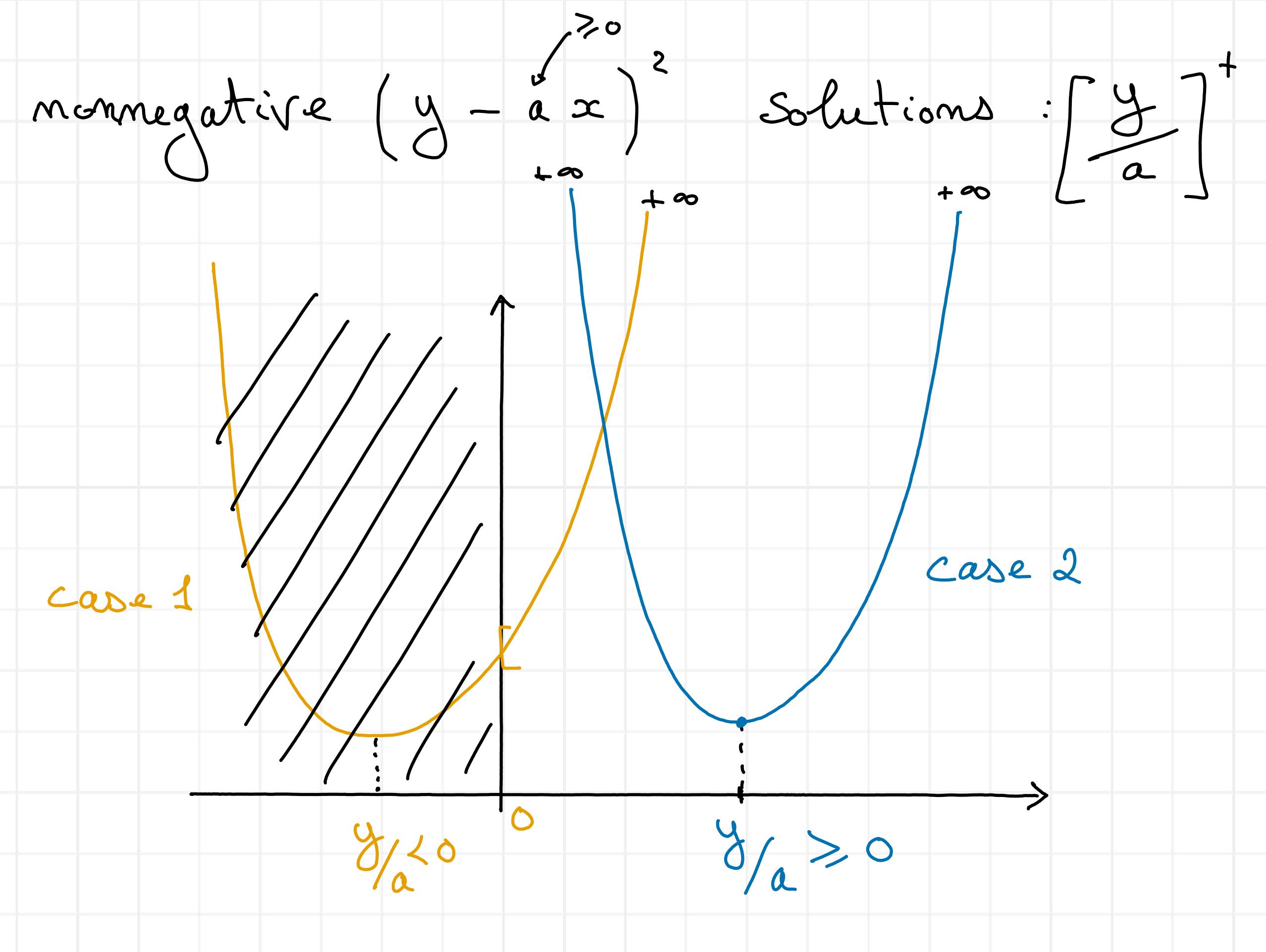
Fig. 18 Solutions to nonnegative least squares in 1d with positive terms.#
HALS uses this strategy over each row \(j\) of matrix \(H^T\), solving iteratively problem (1) with \(Z = Y - W[:,-j]H^T[-j,:]\) and \(w = W[:,j]\). Because each update is an exact minimization procedure, HALS is an instance of exact alternating optimization. As long as each block update is uniquely defined, which happens when \(W\) has nonzero columns, convergence to the global minimizer is ensured; see Alternating optimization. A simple implementation of HALS is provided below, and is also available in tensorly. The input of the algorithm is the grammians \(W^TW\) and \(W^TY\) to utilize faster inner products for high-order tensors.
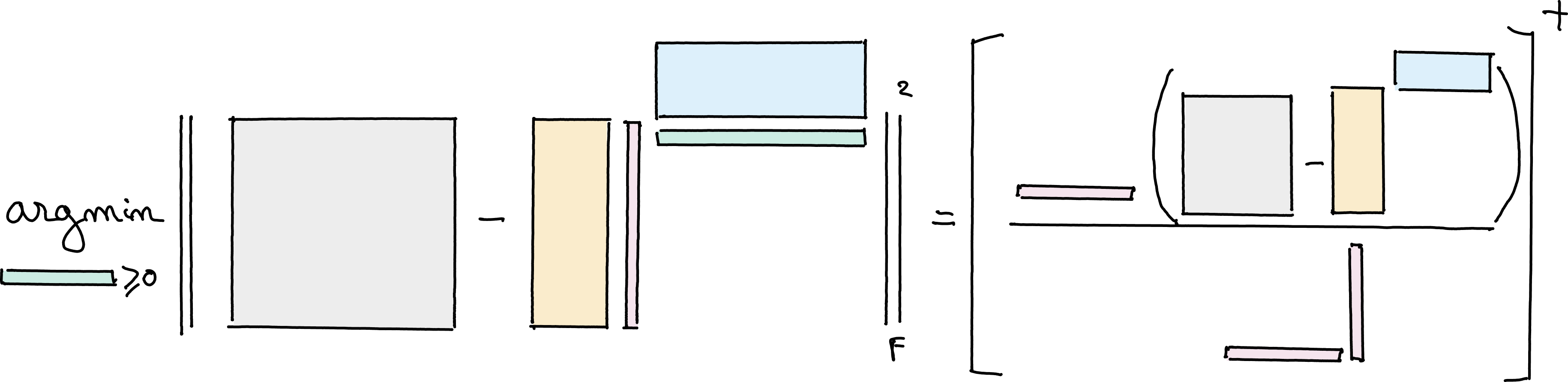
Fig. 19 HALS algorithm principle.#
import tensorly as tl
import matplotlib.pyplot as plt

# Note that HT in the code stands for H^T

def hals_nnls(WtY, WtW, HT=None, n_iter_max=500, tol=1e-8, epsilon=0.0, callback=None):
   rank, _ = tl.shape(WtY)
   if HT is None:
      HT = tl.solve(WtW, WtY)
      HT = tl.clip(HT, a_min=0, a_max=None)

   # For error computation, since W and Y are not known directly
   if callback is not None:
      callback(HT)

   for iteration in range(n_iter_max):
      for k in range(rank):
         if WtW[k, k]:
            num = WtY[k, :] - tl.dot(WtW[k, :], HT) + WtW[k, k] * HT[k, :]
            den = WtW[k, k]
            HT[k,:] = tl.clip(num / den, a_min=epsilon)

      if callback is not None:
         callback(HT)

   return HT
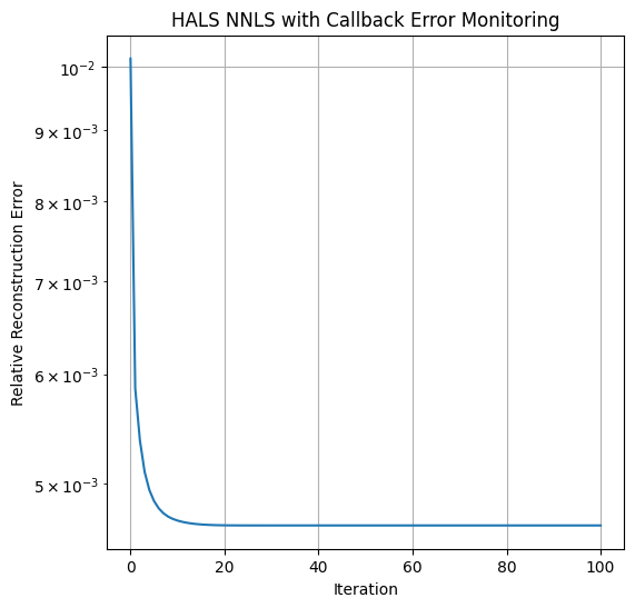
Here is a small example of HALS running on a synthetic matrix NNLS problem. We also show how to use a callback error function to compute reconstruction errors inside the HALS algorithm.
np.random.seed(2)
m=10
r = 6
n=20
W = np.random.rand(m,r)
HTtrue = np.random.randn(r,n) # H^T
HTtrue[HTtrue<0] = 0  # sparsify true H
Y = W@HTtrue + 0.01*np.random.randn(m, n)
errs = []
def callback_err(HT):
   errs.append(np.linalg.norm(Y - W@HT)/np.linalg.norm(Y))
   return True
HTest = hals_nnls(W.T@Y, W.T@W, n_iter_max=100, tol=1e-6, callback=callback_err)
print(f"Relative Reconstruction error: {np.linalg.norm(Y - W@HTest)/np.linalg.norm(Y)}")
print(f"Root mean squared error on H: {np.linalg.norm(HTtrue - HTest)/np.sqrt(r*n)}")

plt.figure(figsize=(6,6))
plt.semilogy(errs)
plt.xlabel("Iteration")
plt.ylabel("Relative Reconstruction Error")
plt.title("HALS NNLS with Callback Error Monitoring")
plt.grid()
plt.show()
Relative Reconstruction error: 0.00466666065517139
Root mean squared error on H: 0.010340649769157119
Multiplicative Updates#
One of the most well-known iterative solvers for general nonnegative least squares problems (both NNLS and NNKL although it is primarily used for the latter) is the MU algorithm. The history of MU is complex. It has been proposed independently under various names in the literature; the oldest reference of MU that I am aware of is probably the so-called Richardson-Lucy iteration [Lucy, 1974, Richardson, 1972], which is specialized for convolutive models and stems from the computational imaging community. MU is also sometimes referred to as the Maximum-Likelihood-Expectation-Maximization (ML-EM) algorithm [Dempster et al., 1977, Fessler and Hero, 1994] as it can be formulated as a particular case of the generic EM framework. MU was popularized in the source-separation community as an algorithm for solving NMF by Lee and Seung in several seminal papers [Lee and Seung, 1999] and was later generalized by Févotte and Idier for a wider class of loss functions [Févotte and Idier, 2011].
The general equations for the MU are, for the NNLS problem,
and for the NNKL problem,
These updates can be derived from several frameworks, as already underlined for the quadratic case in Gillis’s book on NMF [Gillis, 2020]. However, for NNKL, it is important to note that MU is a special case of the EM algorithm; this fact is known to experts in NMF but not to practitioners in computational imaging, where EM for NNKL was originally derived. Below, I therefore provide a brief explanation of how to obtain MU from these various frameworks and the implications of these derivations.
As a gradient ratio#
A simple way to obtain MU is to note that the multiplicative term is the ratio of the negative to the positive parts of the gradient. The gradients are easily computed as
Note that the terms \(W^TWx, W^Ty, W^T\frac{y}{Wx}\) and \(W^T1_n\) are all nonnegative. Denoting \(\nabla_x^{+}\) the positive terms in the gradient computation and similarly for \(\nabla_x^{-}\), we may write rewrite the MU updates as
This interpretation of MU is, in my opinion, useful mostly to quickly remember the updates. While Gillis [Gillis, 2020] provides an interpretation of the gradient ratio related to the KKT conditions (namely, the ratio should get closer to one to satisfy the KKT conditions), deriving convergence results from this formulation is not straightforward. It is also unclear how this update rule will behave for regularized NNLS/NNKL problems.
As a preconditioned gradient descent algorithm#
MU for NNLS can be cast exactly as a preconditioned descent algorithm with a diagonal preconditioner designed to upper-bound the true Hessian. The full description of this formulation is deferred to the second part of the manuscript since it deeply connects with a contribution regarding fast algorithms for NNLS and NNKL.
As a majorization-minimization algorithm#
The MU algorithm was introduced in the source separation and machine learning communities by Lee and Seung in 1999 [Lee and Seung, 1999] as a majorization minimization algorithm. We follow in this paragraph the derivations of Févotte and Idier [Févotte and Idier, 2011] that work for the more general class of \(\beta\)-divergences. For simplicity, we restrict the presentation to the case of a convex loss function for \(\beta\in[1,2]\). We show in the next paragraph that, for the particular case of KL-divergence, the Majorization-Minimization (MM) derivations fall within the EM framework.
The main idea of MM is to fix a current iterate \(x^{(k)}\), build a global majorant of the cost \(\xi(x,x^{(k)})\leq f\left(y,x\right)\) tight and tangent to the cost at \(x^{(k)}\), and then minimize this cost.
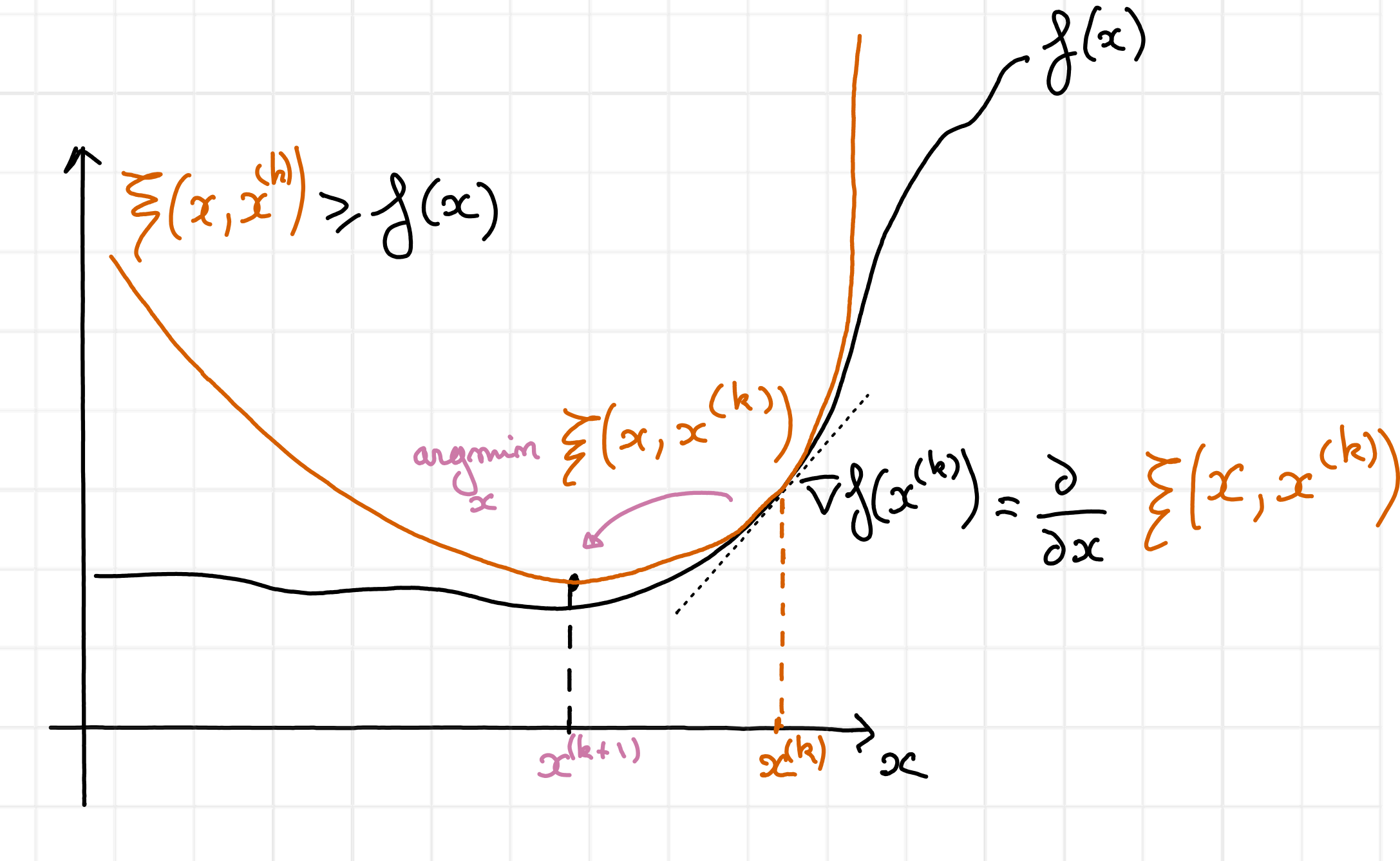
Fig. 20 MM is an algorithmic framework that succesively majorizes a cost function \(f\) globally, and then minimizes the majorant. In this figure, the majorant \(\xi(x,x^{(k)})\), in red, is tight and tangent at the point \(x^{(k)}\). Its minimum is attained at \(x^{(k+1)}\), in purple.#
To obtain the MU algorithm, one may use the convexity inequality for the loss function, also called the Jensen inequality in this context:
for nonnegative coefficients \(\lambda_i\) that sum to one and any positive vector \(x\in\mathbb{R}^{n}_+\). The trick to obtaining MU using MM is to choose the specific values
The estimated observations at the current iterate \(\hat{y} = Wx^{(k)}\) have been introduced to simplify the presentation. The lambda parameters are introduced in the summand of the second argument of the loss, setting \(\sum_j W[i,j] x[i,j] = \sum_j W[i,j]x[j] \frac{\lambda_{i,j}}{\lambda_{i,j}}\). Applying the convexity inequality after observing that \(\frac{W[i,j]}{\lambda_{i,j}}=\frac{\hat{y}[i]}{x^{(k)}[j]}\) yields a majorant of the cost
This majorant is separable and convex, so we can find its minimizer by setting the derivative with respect to each \(x[j]\) to zero. Denoting \(\frac{\partial}{\partial x_2}f\) the partial derivative of the function \(f\) with respect to its second argument, the MM algorithm updates \(x\) by solving
For the Euclidean loss and the KL-divergence, respectively,
both of which, when plugged into the stationary point equation (4), boil down to the MU updates (2) and (3).
The MM interpretation of MU is useful because it automatically guarantees that MU iterations always decrease the cost. Moreover, for NNLS with positive initialization, MU falls within the scope of the SUM framework, which guarantees convergence of the cost to a stationary point. However, additional hypotheses are required to guarantee that the limit point of the cost and the iterates are respectively stationary points and global minimizers of the cost function in the NNKL problem. These assumptions are summarized in [Gillis, 2020], and revolve around the fact that Lipschitz continuity of the cost is required to avoid arbitrarily small improvements of the iterates for a given cost decrease.
Positivity constraints
A workaround for the NNKL problem, that also guarantees the positivity required for convergence in NNLS, is to impose positivity constraints by introducing \(\epsilon>0\) such that \(x\geq \epsilon\). Positivity avoids the non-Lipschitz smoothness of the KL-divergence at zero, and avoids the zero-locking phenomenon [Takahashi and Hibi, 2014]. The MU iterates become
for the NNLS problem, and
for the NNKL problem, where the maximum is applied elementwise. The underlying algorithm here can be thought of as a generalized proximal gradient or preconditioned forward-backward algorithm; see, for instance, the variable metric forward-backward framework for more details [Chouzenoux et al., 2014, Chouzenoux et al., 2016].
As an EM algorithm#
In the MM description of MU, the particular choice for the parameters \(\lambda_{i,j}\), which is crucial to obtain the updates, could seem somewhat arbitrary. It turns out that using the EM framework for the NNKL problem, one can make sense of this choice. Below, we derive MU from EM in a way that slightly differs from earlier references from computational tomography [Dempster et al., 1977] that I find personally hard to follow.
A statistical description of the NNKL problem is required to write the EM algorithm. We suppose that the data samples \(y[i]\) are sampled independently from random variables \(Y[i]\) following Poisson distributions conditionally to the knowledge of unknown parameters \(x\), that is
The MLE in this setting finds the parameters \(x\) that maximize (minimize) the (negative) log-probability of the observations \(y\),
where the summation over \(i\) is due to the independence of the random variables in \(Y\). For the Poisson distribution, one may observe that the log-likelihood is the KL-divergence up to constant terms with respect to \(x\):
Therefore, computing the MLE amounts to solving the NNKL problem.
Basics of the EM algorithm#
EM is a particular case of a majorization-minimization algorithm applied to a log-likelihood. There are several ways to understand EM besides the usual textbook presentation (including MM, proximal point algorithms, alternating optimization); see, for instance, the discussion in [Kunstner et al., 2021]. The MM point of view connects EM with other optimization algorithms quite naturally; let us derive EM within the MM framework.
EM can be obtained by combining two techniques: marginalization with respect to user-chosen latent variables and Jensen’s/convexity inequality (similar to the derivations of MU within the MM framework) to approximate the cost. Introducing latent random variable(s) \(Z\) taking values \(z\) in the set \(\mathcal{Z}\) and the observation vector \(y\), using the total probability law, the log-likelihood writes
These latent variables can represent, for instance, intermediate values in the optimization problem (see the application of EM to NNKL below), or missing observations. A core idea of EM (and more generally variational Bayesian estimation) is to leverage Jensen’s inequality to build a lower bound of \(\log p(y ~|~ x)\) by introducing another well-chosen distribution. EM is an iterative algorithm in which, at iteration k, this distribution is chosen as \(p(z ~|~ y, x^{(k)})\), which is, in essence, the distribution of the latent variables given the observed data and the current estimates of the unknown parameters. In many cases, this conditional distribution can be derived from the statistical description of the problem. More precisely, the log-likelihood is lower-bounded as follows:
One can also easily show that this lower bound is tight for \(x=x^{(k)}\) and that the first-order derivatives match. To minimize the negative log-likelihood, the EM algorithm therefore minimizes \( \mathbb{E}_{z | y, x^{k}}\left[ -\log p(y,z ~|~ x) \right] \) with respect to \(x\). There are again many other equivalent formulations of the functional minimized by EM. One that works well for source separation problems is to introduce back the conditional likelihood and prior information on the latent variables:
Thus far, the EM algorithm is rather high-level and abstract. One personal difficulty in applying EM has always been to make sense of the probabilities and the conditional expectation in (5). For some problems, deriving these quantities can in fact be very challenging. Hopefully, this is not the case for NNKL, and the EM algorithm is derived in the next section.
Relationship between EM, MU, and mirror descent
Bauschke, Bolte, and Teboulle have proposed to solve NNKL using (proximal) mirror descent [Bauschke et al., 2017]. They make use of a particular choice of potential, Burg’s entropy \(-\sum_i\log(x[i])\), and show that KL-divergence is smooth relative to this choice with constant \(\frac{1}{\|y\|_1}\). In other words, KL-divergence can be upper-bounded using a first-order approximation and the Bregman divergence \(\mathcal{D}_h\) obtained with Burg’s entropy
\( \KL{y,Wx} \leq \KL{y,Wx^{(k)}} + \langle \nabla_x\KL{y,Wx^{(k)}}, x - x^{(k)} \rangle + \frac{1}{2\|y\|_1}\mathcal{D}_{h}(x,x^{(k)}),\)
that yields, after simple derivations found in [Bauschke et al., 2017]
\( \KL{y,Wx} \leq \KL{y,Wx^{(k)}} + \langle W^T\left(1_n-\frac{y}{Wx^{(k)}}\right), x - x^{(k)} \rangle + \frac{1}{2\|y\|_1} \sum_{j\leq n} \frac{x[j] - x^{(k)}[j]}{x^{(k)}[j]} - \log\frac{x[j]-x^{(k)}[j]}{x^{(k)}[j]}.\)
Minimizing this upper-bound leads to unusual multiplicative updates
\( x = x \ast \frac{1}{1+\frac{1}{\|y\|_1}x \odot \left(W^T1_n - W^T\frac{y}{Wx}\right)}. \)
Since these updates allow the use of (Bregman) proximal operators while ensuring convergence, they have been used in regularized NNKL problems [Hurault et al., 2023]. However, it is unclear how these updates compare to the classical MU (3) and its convergence rate is unknown.
Recently, a formal link was established between the EM algorithm for the exponential family [Kunstner et al., 2021] and mirror descent with Bregman divergences. It allows, in particular, the derivation of linear convergence rates for EM, and therefore for the usual MU in the NNKL problem. This also shows that other choices of potential, besides Burg entropy, lead to interesting update rules for NNKL. This was brought to my attention by Thibaut Modrzyk, who is currently investigating this observation. The relationship between MU and mirror gradient descent was also partially discussed in [Hien and Gillis, 2021] . Linear convergence of NNKL explains why the MU algorithm is an efficient method for solving NNKL.
MU is an instance of EM for NNKL#
To apply EM to NNKL, on top of introducing the Poisson distribution on the observed variables \(Y[i]\), we introduce latent variables that will allow us to derive the EM algorithm efficiently. The literature [Dempster et al., 1977, Shepp and Vardi, 1982] informs us to define independent latent variables
such that \(\sum_{j\leq n} Z[i,j] = Y[i]\). In source separation, random variables \(Z[i,j]\) model (parts of) the various components in an additive mixture and therefore bear physical meaning.
We can now expand the upper-bound \(\xi\). First notice that the prior distribution of the latent variables \(p(z ~|~ x)\) is separable into the product \(\prod_{i,j} p(z[i,j] ~|~ x[j])\) since all latent variables are mutually independent, and the random variable \(Z[i,j]\) depends only on the parameter \(x[j]\). Therefore,
The conditional likelihood \(p(y[i] ~|~ z[i,:], x)\) has a particular shape. Because we defined the latent variables \(Z\) such that \(Y[i] = \sum_j Z[i,j]\), conditionned on \(Z\), \(Y\) is deterministic. To simplify, we thereafter treat this first term in the majorant as a constraint imposing that the latent variables indeed sum up to the observations, \(y[i] = \sum_j Z[i,j]\) (otherwise the logarithm goes to \(-\infty\)), and ignore it in the definition of the cost. Therefore,
After expending the priors,
the upper-bound simplifies into
The last term involving the factorial of the latent variables is constant with respect to the parameters \(x\) and can be ignored. What remains to compute to obtain a simpler form for the majorant \(\xi\) is the expected value of \(Z[i,j]\) conditioned to the knowledge of the sum of other Poisson variables \(\sum_j Z[i,j]\) and the parameter values \(x^{k}\) of the Poisson laws, \(\mathbb{E}_{Z[i,:] |y[i], x^{k}}\left[z[i,j]\right]\) with \(y[i]=\sum_j Z[i,j]\).
The following Lemma allows us to conclude, its proof is simple [van Oosten, 2014].
Lemma 1 (Distribution of Poisson variables conditionned by their sum)
Let \(Z_1, Z_2\) be two random variables distributed respectively as \(\mathcal{P}(\lambda_1)\) and \(\mathcal{P}(\lambda_2)\). Then the conditionned random variable \(Z_1 | Z_1+Z_2\) follows a Binomial distribution \(\text{Bin}(Z_1+Z_2,\frac{\lambda_1}{\lambda_1+\lambda_2})\).
Applying Lemma 1 with \(Z_1 = Z[i,j]\) and \(Z_2 = y[i] - Z[i,j]\) yields
Notice that we recover the weights of the MM formulation of MU, \(y[i]\lambda_{i,j} = \mathbb{E}_{Z[i,:] | y[i], x^{k}}\left[z[i,j]\right]\), which provides a nice interpretation of the ad-hoc choice for these parameters in the MM framework for NNKL.
We now observe that the majorant \(\xi\) is equal up to constant terms to the majorant obtained with the MM framework, and the gradients of the two convex separable majorants match:
Therefore, the EM algorithm for NNKL is exactly MU.
MU may not be an instance of EM for NNLS#
Importantly, while the EM algorithm can in principle be used to derive update rules for the NNLS problem given reasonable additional statistical assumptions on the variance of the variables \(z[i]\), the update rules obtained with these assumptions on distributions do not match the MU updates (2). Instead, they are another particular case of diagonally preconditioned gradient descent; see, for instance, [van Oosten, 2014].
Equivalence of the MU formulations breaks with l1 and l2 regularizations
If additive \(\ell_1\) and \(\ell_2\) regularizations terms \(\lambda_1 \|x\|_1 + \frac{1}{2}\lambda_2 \|x\|_2^2\) are added to the cost, the MU updates using the gradient ratio for both NNLS and NNKL would write
since the gradients of the regularizations are always positive. For instance, for NNKL, MU obtained from the gradient ratio heuristic is
However, using the MM framework, the impact of the regularizations on the update rules changes for NNLS and NNKL. Note that a more complete analysis is provided in [Leplat et al., 2021]. The updates within the MM framework are given by solving
Injecting the gradients of the cost function yields
and the resulting MU updates for the NNLS problem are
Note the difference with the gradient ratio heuristic that places the \(\ell_1\) regularization hyperparameter in the denominator. Moreover, these MU updates with \(\lambda_1\geq 0\) can in principle become negative or zero; therefore, positivity constraints should be enforced as discussed above.
For the NNKL problem, one needs to compute the positive roots of the second-order polynomials
Best nonnegative rank-one approximations#
We have mainly focused in this section on solving nonnegative regression problems. We will discuss algorithms for LRA throughout the rest of this manuscript, with a particular focus on alternating algorithms in Alternating optimization. However, there exist closed-form algorithms for the best rank-one nonnegative approximation, related to the discussion of NNLS and NNKL.
KL-divergence NMF#
Consider the rank-one NMF approximation problem in the KL-divergence
The optimal scaling condition imposes that
We immediately deduce that solutions \(h^\ast\) and \(w^\ast\) are proportional to the marginals of the observation matrix \(Y\). If we further assume that both vectors have the same scales, the closed-form solution writes
In other words, the best nonnegative rank-one approximation in the KL-divergence is known in closed form, and its computation is straightforward. This result has probably been known for a long time, as it is related to the Sinkhorn algorithm [Sinkhorn and Knopp, 1967], to the estimation of coupled probabilities, and to information-geometric concepts [Ghalamkari et al., 2025]. It has been introduced in the NMF community several times, in [Ho and Van Dooren, 2008] and in [Huang and Sidiropoulos, 2017]. The analogy with the scaling problem and the Sinkhorn algorithm in particular can be seen by noticing that
and that the Sinkhorn algorithm can be used to solve the optimization problem
that is, scaling a matrix \(X\) to have the same marginals as another given matrix \(Y\). In general, this problem has no closed-form solution.
Frobenius norm NMF#
Computing the best rank-one approximation in the Frobenius norm, that is, solving
in general is NP-hard [Gillis and Glineur, 2014]. However, for nonnegative data \(Y\in\mathbb{R}_+^{m\times n}\), the solution can be computed efficiently (in particular, in polynomial time) using a rank-one Singular Value Decomposition. Indeed, for positive matrices, the Perron-Frobenius theorem guarantees that the first singular vectors and the first singular value are always positive. If the data has zero entries, the Perron-Frobenius theorem does not hold in general, but it has been shown that the solution can still be obtained using the absolute values of the first components. Indeed, following [Gillis, 2020]:
and by optimality of the SVD, for any couple \((w,h)\) (in particular with nonnegative entries),
We have therefore found an admissible solution with the lowest possible cost.