
One-sparse dictionary-based LRA#
Reference
[Cohen and Gillis, 2018] J. E. Cohen, N. Gillis, “Dictionary-based Tensor Canonical Polyadic Decomposition”, IEEE Transactions on Signal Processing, vol.66 issue 7, pp. 1876-1889 2018. pdf
Note
Out of simplicity, we present only the matrix case, but both one-sparse dictionary-based matrix and tensor low-rank decompositions are studied in our work [Cohen and Gillis, 2018]. In particular, we demonstrate that one-sparse DLRA is a well-posed approximate tensor decomposition problem, in contrast to approximate CPD. Also note that this work has been studied against global optimization solutions in 2023 [Dache et al., 2023].
We are interested in solving the following matrix factorization problem:
where \(\Omega_B\) is typically \(\mathbb{R}^{n\times r}\) or \(\mathbb{R}^{n\times r}_+\) with \(r\leq m,n\).
This problem, coined one-sparse DLRA, consists of finding the columns of the dictionary \(D\) indexed in the set \(\mathcal{K}\) such that the data matrix \(Y\) is well approximated by a low-rank model \(D[:,\mathcal{K}]B^T\). One can also rewrite one-sparse DLRA using a selection binary matrix \(S\) whose columns have a single nonzero element at each \(\mathcal{K}[q]\) for \(q\in[1,r]\), this yields \(D[:,\mathcal{K}]B^T=DSB^T\).
The code snippet below shows how to generate such a data matrix \(Y\) without noise. We use a hyperspectral image available in tensorly.dataset, and assume that a few pixels are pure. This means that the source matrix \(A\) is contained in the data itself; in other words, \(A=D[:,\mathcal{K}]\) but \(\mathcal{K}\) is unknown.
import numpy as np
import tensorly as tl
from tensorly.datasets import data_imports
import matplotlib.pyplot as plt
from tensorly_hdr.image_utils import convert_to_pixel, convert_to_index

# Import an hyperspectral image
image_bunch = data_imports.load_indian_pines()
image_t = image_bunch.tensor # x by y by wavelength
image_t = image_t/tl.max(image_t) # maximum value set to 1

# Vectorize the tensor into a m\times n matrix (wavelength \times pixels, y vary first)
image = tl.unfold(image_t, 2)

# Simulation parameters
# For illustration purposes, we can pick a few spectra and build a synthetic data matrix accordingly.
band = 70
rank = 3
# hand-picked road, field, and forest
Kx = [70,40,10]
Ky = [62,100,100]
K = convert_to_index(Kx, Ky, image_t.shape[1])
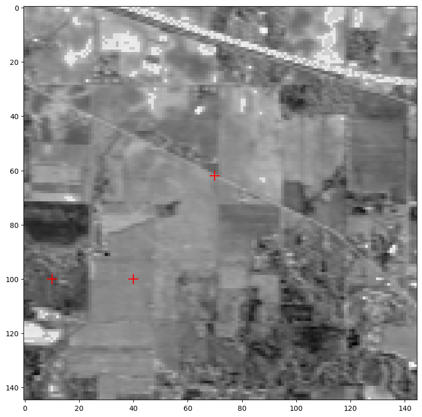
Showing the hyperspectral image at band indexed by 70
Red crosses signal the position of the hand-picked pure pixels
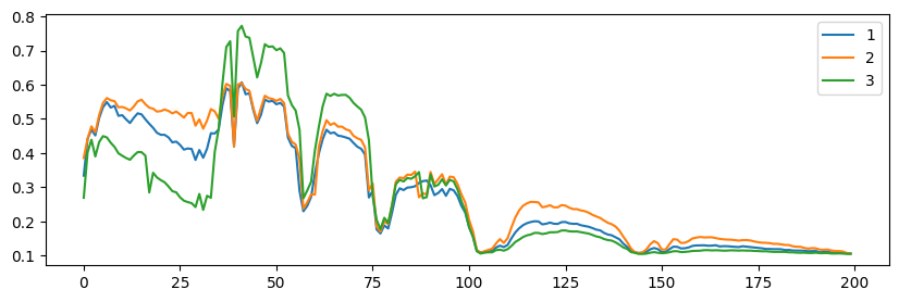
Showing 3 pixels (spectra) indexed by [9060, 14540, 14510]
from tensorly_hdr.image_utils import sparsify
Bt = np.random.rand(rank, image.shape[1]) # elementwise nonnegative
# We sparsify B so that not all pixels use all three spectra, this is optional
Bt = sparsify(Bt, s=0.5)
Y = image[:,K]@Bt
The columns of the matrix \(Y\) are now indeed linear combinations of only three columns in the dictionary \(D\) (which is the original hyperspectral image itself in this particular case). The DLRA problem consists of finding the pure pixel indices \(\mathcal{K}\) and the abundances \(B^T\).
Note
The one-sparse DLRA model under scrutiny in this section has strong connections to other matrix and tensor factorization models, most prominently Multiple Measurements Vector (MMV), also known as collaborative sparse coding. The main different is that MMV does not assume that the data is low-rank. On the other hand, MMV transforms the bivariate problem into a single convex problem over the \(SB^T\) matrix, which can be solved optimally but typically involves significantly more variables and requires guarantees for the correctness of the convex relaxation.
Identifiability of one-sparse DLRA#
There are at least two questions of interest regarding one-sparse DLRA:
In general, low-rank approximations are not interpretable because of the rotation ambiguity. For the one-sparse DLRA model, does the sparsity constraint lead to identifiability?
May an algorithm be designed that finds optimal solutions in a reasonable time?
We first answer the identifiability question positively under mild conditions on the dictionary.
Theorem 14
Let \(Y\) be a real \(m\times n\) matrix of rank \(r\), and let \(D\) be a real \(m\times d\) matrix with \(\text{spark}(D)>r\). If there exists a full column rank permutation matrix \(S\) (columns are one sparse and entries are binary) and a matrix \(B\in\R{n\times r}\) with nonzero columns such that \(Y=(DS)B^T\), then \(S\) and \(A\) are unique up to permutation ambiguity.
See [Cohen and Gillis, 2018] for the proof.
In other words, for a well-built dictionary with incoherent atoms, the dictionary constraint leads to uniqueness of the matrix factorization problem.
A simple heuristic for one-sparse DLRA#
Designing an optimization algorithm with performance guarantees for one-sparse DLRA is not straightforward since one-sparse DLRA is a generalization of sparse coding (sparse coding is recovered when \(n=1\)). While we can consider convex relaxations for the sparsity constraints, empirically, we found that a heuristic based on ALS works rather well. In what follows, we introduce this heuristic, which we coin Maximum Correlation ALS (MC-ALS), and showcase its performance in spectral unmixing. However, we defer the formal analysis of MC-ALS performance to the k-sparse DLRA problem.
MC-ALS works as follows: we view the submatrix \(D[:,\mathcal{K}]\) as factor matrix \(A\), and compute the least squares estimate
If, in the application at hand, the matrix \(A\) is nonnegative (like the spectra of our running hyperspectral image example), we may use a NNLS solver instead.
Then given an estimation \(\hat{A}\), the closest atom in the dictionary \(D\) is computed for each column of \(\hat{A}\)
Note
Using the largest absolute scalar product between the atoms and the estimated factor matrix \(\hat{A}\) may lead to selecting the same atom twice, e.g., if two columns of \(\hat{A}\) are similar. This problem can be alleviated by rather selecting indices \(\mathcal{K}\) as the optimal linear assignement of atoms in the dictionary \(D\) to columns of matrix \(\hat{A}\):
This problem is solved efficiently using, for instance, the Hungarian algorithm [Kuhn, 1955]. In the original work [Cohen and Gillis, 2018], we did not use a linear assignment problem solver, but we do here because it avoids the singularity of the estimated factor.
This yields the following routine to estimate the matrix \(A\) given an estimate of matrix \(B\).
from scipy.optimize import linear_sum_assignment
# scipy is a dependency of tensorly

def MC_ALS_Aestimation(Y, D, B, nonnegative=True):
    # Should ensure the dictionary has normalized columns
    if nonnegative:
        Ahat = tl.solvers.hals_nnls(B.T@(Y.T), B.T@B, n_iter_max=20).T
    else:
        Ahat = tl.solve(B.T@B,B.T@(Y.T)).T
    K, _ = linear_sum_assignment(tl.abs(D.T@Ahat), maximize=True)
    Ahat2 = D[:,K]
    return K, Ahat2, Ahat

D = image/np.linalg.norm(image,axis=0)
B = Bt.T
out = MC_ALS_Aestimation(Y, D, B)
print(f"Selected pixels by MC-ALS: {list(out[0])}, ground truth: {K}")
Selected pixels by MC-ALS: [np.int64(9060), np.int64(14510), np.int64(14540)], ground truth: [9060, 14540, 14510]
In the code snippet above, we can recover the indices of the atoms that we hand-picked earlier. However, we assumed that the matrix \(B\) is known, and no noise was added to the system.
The full algorithm requires estimating the matrix \(B\). Because we work here with hyperspectral images and both spectra and abundances are nonnegative, we use a NNLS solver to estimate \(B\) rather than ordinary least squares.
def MC_ALS(Y, D, B_0, itermax=100):
    errs = []
    B = np.copy(B_0)
    for it in range(itermax):
        # estimate A
        K, A, _ = MC_ALS_Aestimation(Y, D, B)
        # estimate B
        #B = tl.solve(A.T@A, A.T@Y).T
        B = tl.solvers.hals_nnls(A.T@Y, A.T@A, n_iter_max=20).T
        # compute error
        errs.append(tl.norm(Y - A@B.T)**2/tl.prod(Y.shape))
        # stop if error has not changed at all (algorithm is stuck)
        if it>1 and errs[-2]==errs[-1]:
            print("Final estimated indices", K)
            print("MSE", errs[-1])
            break
    return (None, [A, B]), errs, K

out = MC_ALS(Y, D, np.random.rand(*B.shape))
Final estimated indices [ 4116 14510 14540]
MSE 7.657730822083651e-06
We can compare the indices of the atoms selected by MC_ALS with the (synthetic) ground truth.
print(K, out[2])
[9060, 14540, 14510] [ 4116 14510 14540]
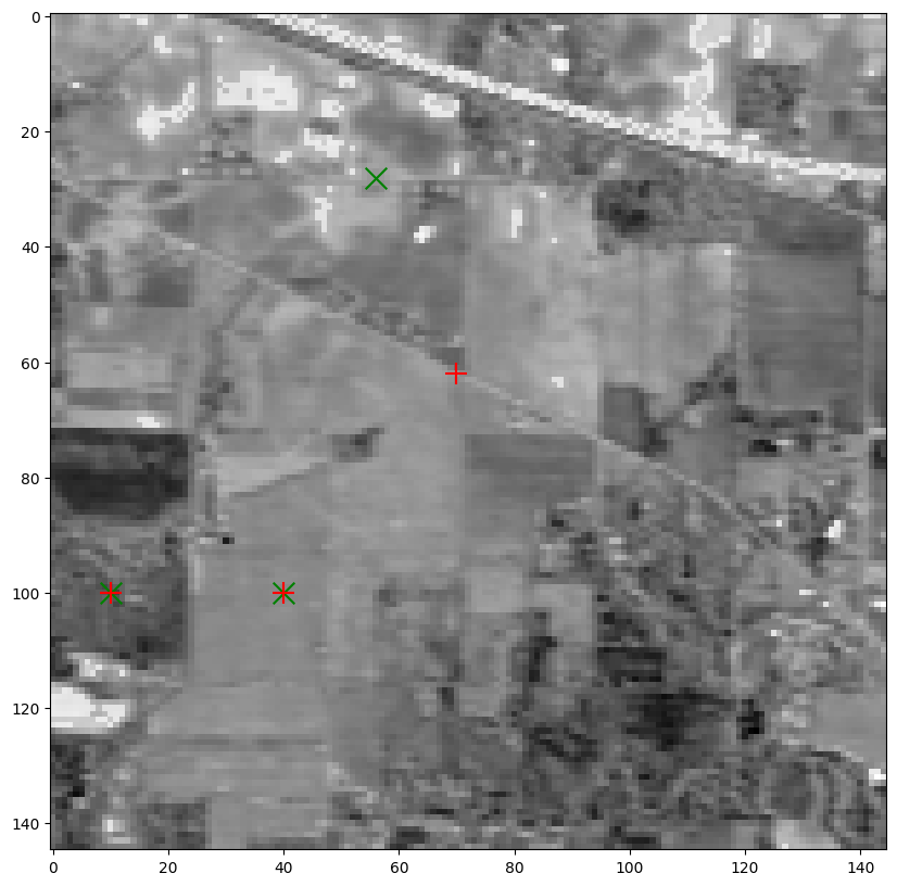
If one runs the experiment several times, one might observe that the ground truth is often only partially recovered, even in the absence of noise. Moreover, the results are surprisingly consistent across runs. We can place the selected pixels on the hyperspectral image (in green) and plot the corresponding spectra. Notice how the selected pixels sometimes still appear to belong to the same class as the ground truth (road, forest, field).
Kxe, Kye = convert_to_pixel(out[2], image_t.shape[1])
plt.figure(figsize=(12,10))
plt.imshow(image_t[:,:,band], cmap="Greys")
# Also showing the pixels we hand-pick as pure
plt.scatter(Kxe, Kye, s=200, c='green', marker='x')
plt.scatter(Kx, Ky, s=200, c='red', marker='+')
plt.show()
# Show spectra from selected pixels
plt.figure(figsize=(10,3))
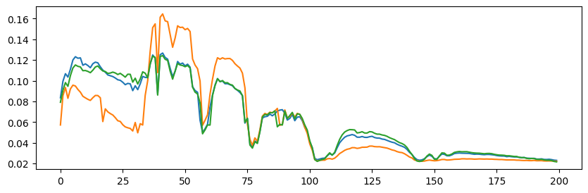
print(f"Showing {rank} pixels (spectra) indexed by {out[2]}")
plt.plot(out[0][1][0])
plt.show()
Showing 3 pixels (spectra) indexed by [ 4116 14510 14540]
A common issue with MC-ALS is that the algorithm often gets stuck after only a few iterations. Indeed, during an iteration in which \(A\) changes slightly but the selected atoms remain the same as in the previous iteration, the estimates \(A\) and \(B\) are identical to those of the previous iteration. We can tackle this issue by using a more flexible formulation or a convex relaxation, but, in our experience, the empirical performance of these variants is similar or worse. This phenomenon can be observed in the toy experiment above; see below the printed number of iterations before the MC-ALS algorithm got stuck.
Number of iterations of MC-ALS: 7