
Applications of rLRA: summary#
Regularizations in LRA are necessarily driven by the properties of the low-rank factors one seeks to recover from the computation of LRA. Therefore, by understanding the applications of LRA in signal processing, one can derive both interesting fundamental problems related to LRA and ideas for designing regularizations and algorithms. Conversely, in some applications, such as medical imaging, theoretical guarantees on the quality of the reconstructed factors in rLRA are important because interpretation errors in these methods’ outputs may have a significant impact. In an optical biopsy application I contributed to, rLRA outputs allow a surgeon to decide whether to remove brain cells during surgery. Removing too few may lead to cancer recurrence, but removing too much may harm critical brain functionalities.
In my work, I have focused on a few specific modalities to gain expert knowledge in these fields and making actually useful practical contributions based on rLRA. The first modality is spectral imaging, both in remote sensing and in microscopy, and the second is music information retrieval, in particular automatic music transcription. Around the end of my PhD, I also worked on chemometrics datasets that included fluorescence spectroscopy [Cohen et al., 2016], chromatography, and nuclear magnetic resonance, which share similarities with spectral imaging in terms of signal processing.
Spectral imaging and rLRA#
Basics of spectral representation of light#
Note
The following paragraphs deal with radiative transfer, a scientific discipline in optics and physics that I am not very familiar with. In particular, I have not read many scientific articles on this topic and have instead used mediation materials, such as those found on Wikipedia. Here are some links for radiative transfer, color, and additive and substractive mixtures.
In everyday life, color helps distinguish different objects and materials in space. Color, in fact, carries a lot of information about our environment: one would probably never eat a light-blue apple because this unusual color is a sign that the apple may contain unwanted chemical components. Tree leaves are typically orange-ish when they dry and are about to fall, but typically green-ish in spring and summer. It is, therefore, a very natural and old idea to exploit color information in science to obtain information on an observable system.
From a mathematical and informatics point of view, defining color formally is, maybe surprisingly, a large and complex research domain. For simplicity, let us assume that colors can be represented in a three-dimensional space using the basis vectors red, blue, and green. Any two-dimensional \(m\) by \(n\) color image is, in this simplistic model, a tensor of size \(m\times n \times 3\).
From a physical perspective, color is not a physical property of matter. It relates to human perception (and therefore varies for each individual) of a physical property called wavelength, which characterizes the distance an electromagnetic wave travels in a single cycle. More precisely, any wave can be decomposed in the spectral domain as the sum of sinusoidal waves with a fixed wavelength. This is exactly the Fourier transform ubiquitous in signal processing. Any light emitted or reflected by a source of interest has a specific spectrum that represents the amplitude of the individual additive sine waves, and which contains information about the source, just like color. In fact, color, as described in the simplified RGB format, is a compressed representation of the full light spectrum, in which spectral coefficients are grouped into three blobs, respectively named red, green, and blue, see Fig. 30. This is mostly due to human perception: while human ears excel at identifying the Fourier coefficients (the amplitude of each additive sinusoidal wave) of air pressure wave, the human eye is much less sensitive; cones in the human eye that are sensitive to color naturally perform this dimensionality reduction.
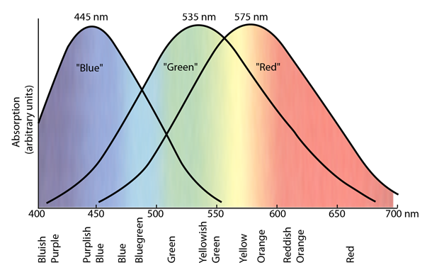
Fig. 30 [From hyperphysics.phy-astr.gsu.edu] “There are three types of color-sensitive cones in the retina of the human eye, corresponding roughly to red, green, and blue sensitive detectors. Painstaking experiments have yielded response curves for three different kind of cones in the retina of the human eye. The “green” and “red” cones are mostly packed into the fovea centralis. By population, about 64% of the cones are red-sensitive, about 32% green sensitive, and about 2% are blue sensitive. The “blue” cones have the highest sensitivity and are mostly found outside the fovea. The shapes of the curves are obtained by measurement of the absorption by the cones, but the relative heights for the three types are set equal for lack of detailed data. There are fewer blue cones, but the blue sensitivity is comparable to the others, so there must be some boosting mechanism. In the final visual perception, the three types seem to be comparable, but the detailed process of achieving this is not known. When light strikes a cone, it interacts with a visual pigment which consists of a protein called opsin and a small molecule called a chromophore which in humans is a derivative of vitamin A. Three different kinds of opsins respond to short, medium and long wavelengths of light and lead to the three response curves shown above. For a person to see an object in color, at least two kinds of cones must be triggered, and the perceived color is based on the relative level of excitation of the different cones.”#
This fact has a few interesting consequences. First, the human eye is blind to wavelengths outside the visible range, limiting our ability to detect spectral information in the infrared or ultraviolet. Second, two objects of the same color can have very different spectra. Therefore, the human eye is a poor spectral sensor. Hopefully, it is possible to accurately measure the light spectra of a single light flux using prisms that have the property to spread light beams spatially depending on the wavelength. In other words, prisms perform, in some way, a Fourier transform of an incoming light wave and output the individual sinusoidal light waves with pure wavelengths separated spatially. It is then possible to measure the spectrum by essentially taking a black-and-white picture of the prism output. Devices that measure light spectra, using prisms or other separation means, are called spectrometers.
Fig. 31 [From Wikipedia, credits Lucas Vieira] An illustration of the dispersion property of a prism. Incomming white light is decomposed as a sum of monochromatic light beams with increasing wavelength.#
Spectral mixing and unmixing#
We are taught in high school that colors obey two sets of rules for mixing: additive and subtractive. Additive mixture works for light and is typically described in the RGB color space: red + blue light yields magenta, red + blue + green light yields white. This principle is ubiquitous in everyday life, since color screens rely on it to generate colors by combining red, blue, and green light from tiny light sources for each pixel. Subtractive synthesis applies, for instance, to paint, typically in CMY format: cyan + magenta yield blue, cyan + magenta + yellow yield black. The coexistence of these two models can be slightly confusing: when is a mixture additive or subtractive? Is it possible to design additive mixtures of paints and subtractive mixtures for light beams?
A way to explain additive and subtractive mixtures, which I find useful, is to relate them to the physical process underlying the mixture and to the full spectral description of color. An additive mixture is a matter of perception. Various light beams with different spectra hit the human eye and are seen as a single light source by the lens, which focuses the input light onto the cones, integrating the contributions of each light source. In the case of a spectrometer, an optical lens can be used to produce a similar additive acquisition. Addition synthesis is therefore not a physical modification of the wavelengths of a light wave, but rather the (spatial) superposition of different light waves. In contrast, a subtractive mixture is a direct modification of the spectrum of a light wave that removes a part of that spectrum. A key concept to understand a subtractive mixture is filtering: when a light wave hits an object, it is partially absorbed and partially reflected. The intensity of reflected light depends on the wavelength. The reflected light has a different spectrum than the input light, filtered by the object’s spectral response. What we usually call the color of an object is, in fact, the projection in RGB space of the resulting spectrum of “white” light after it has been reflected by the item. The absorption spectrum of an object is the spectral filter by which the incoming light is multiplied to obtain the reflected light spectrum. A subtractive mixture is simply the sequential filtering of a light source by several items, where spectral filters are combined multiplicatively. When mixing paints, the chemical compounds in each paint are intimately mixed, and the paint after mixture essentially filters light jointly for all paints.
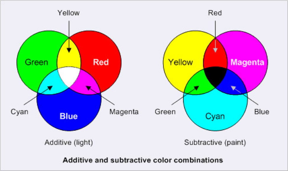
Fig. 32 [From intranet.mcad.edu] An illustration of additive and substractive mixtures. Additive mixture is essentially a property of light, and allows to generate a large range of pure wavelengths in the visible range. Substractive mixture is obtained by spectral filtering and is less expressive in general than RBG.#
In scientific imaging, both additive and subtractive mixtures are usually encountered. The important point is that an additive mixture is usually well-suited to linear models, whereas a subtractive mixture leads to non-linear models. Two examples of additive mixture help illustrate this fact.
a. Fluorescence Spectroscopy in chemometrics. A mixture of several fluorophores is observed with a spectrometer. Each fluorophore emits a light wave with a specific spectrum. Since the fluorophores are loosely mixed within the sample and each emits a fluorescence signal individually, the measured spectrum is simply the sum of the fluorescence spectra of each component. The light emitted by the fluorophores depends on the wavelength of the light exciting the sample; using a laser excitation with a controlled wavelength leads to a series of spectra acquisitions, stored in a matrix (fluorescence excitation emission matrix) \(Y\) with \(n\) columns corresponding to excitation wavelengths and \(m\) rows containing the measured additive mixture of fluorescence spectra. Additive mixture in this context is also related to the Beer-Lambert law, and translates into an (approximate) low-rank NMF
where \(W\) is a matrix containing the spectra of each individual fluorophore in the chemical mixture, and \(H\) contains the amplitude of each fluorophore response to the excitation wavelength. Applying NMF to the data matrix \(Y\), or nonnegative tensor factorization to several such measurement matrices, can in principle recover the individual fluorescence spectra, essentially performing spectral unmixing.
b. The linear mixing model in remote sensing makes the hypothesis that materials on an observed scene are spatially distributed and non-overlapping. The scene is cut into pixels by the camera, and each pixel may therefore contain several materials with proportions given by the portion of the pixel covered by each material. The spectral acquisition is then the additive mixture of the reflectance spectra (the ambient-light spectrum, essentially white, filtered by each material). For a single-pixel \(Y[:,i]\) of the acquired spectral image \(Y\) with \(m\) spectral wavelengths (or spectral bands if spectra are acquired in a compressed spectral representation) and \(n\) pixels, the additive mixture of \(K\) materials simply translates into a linear model
where \(W\) contains columnwise the spectra of each material in the scene (supposing they are consistent over the whole image), and \(H\) contains columnwise the proportions of the materials in each pixel, also called abundances. Extensions of the linear mixing model that account for multiple reflections typically involve products of the matrix \(W\) with itself; this is consistent with the subtractive mixture model, where the ambient light is filtered consecutively by several materials [Kervazo et al., 2021].
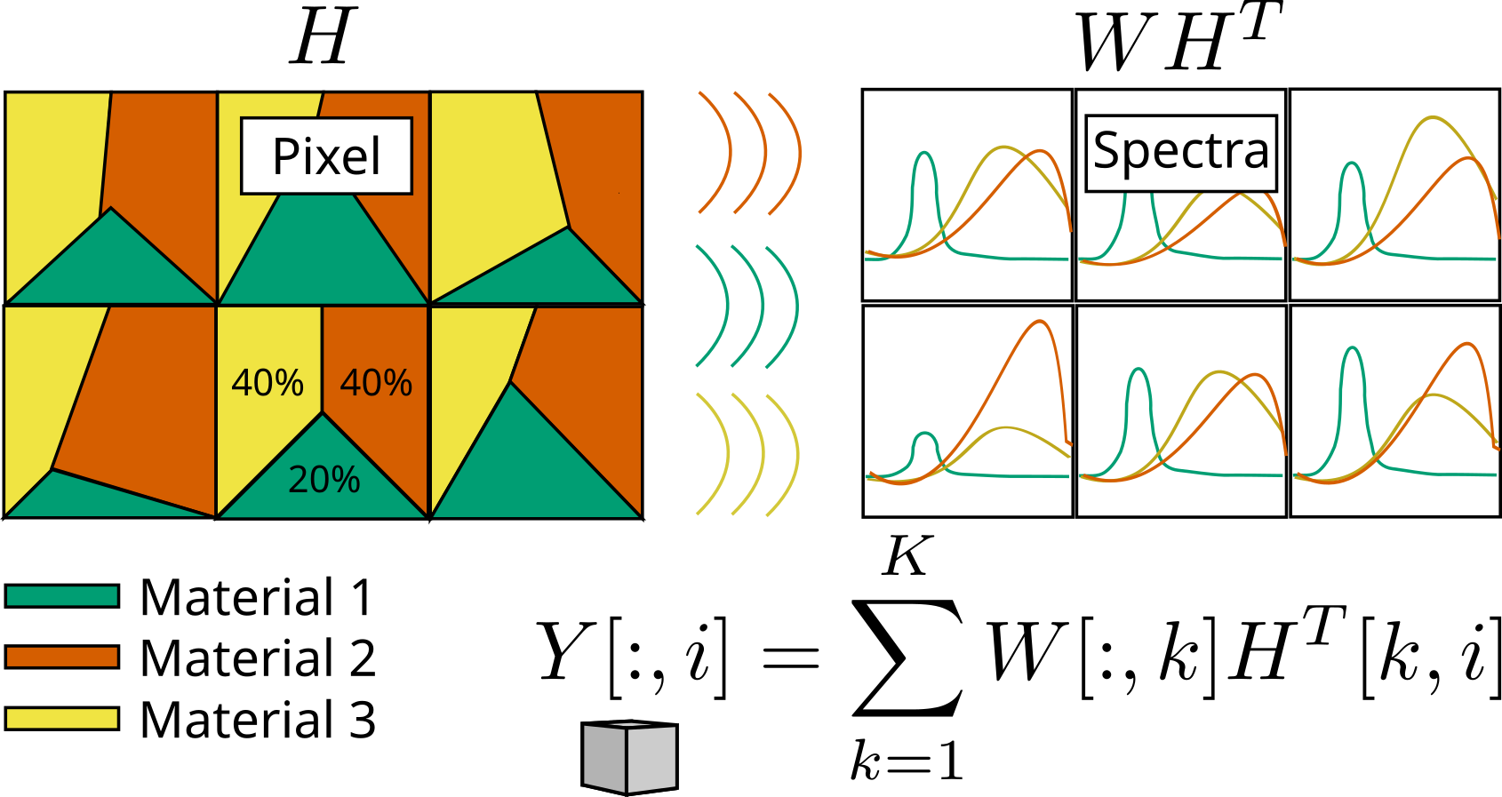
Fig. 33 An illustration of the linear mixing model. Each pixels (squares in the top left grid) have different abundances of each material. This translates into an additive mixture of the spectra contained in matrix \(W\), weighted by these abundances pixelwise.#
To conclude this introduction to spectral unmixing, we can now answer the question above: Is it possible to mix paints additively to produce white? The answer is nuanced. It is impossible to mix paint to produce pure white. Mixing paints intimately will result in a filtering effect that attenuates the ambient light spectrum across all wavelengths, leading to black. However, we can produce grey by juxtaposing paints on a surface and looking from afar. Spatial juxtaposition will result in additive filtering of the filtered white light, as in the linear mixing model. If three paints red, blue, and green are used in equal proportions, the resulting spectrum is the sum of blue, red, and green light but with reduced intensity, and the object will appear gray. Screens can produce white because they can emit red, blue, and green spectra at full intensity, which is not possible with reflectance spectra.
Several applications of spectral unmixing#
Spectral unmixing separates spectra from several acquisitions of additive mixtures with varying mixture conditions. A popular example of spectral unmixing in the signal processing community is found in remote sensing, and I have often motivated rather theoretical works with such images. Since my arrival at CREATIS in 2022, however, my work has focused on optical systems that enable optical biopsy. Optical biopsy is a non-invasive technique that enables the acquisition of spectral information from tissues (e.g., brain cells) during live surgery without requiring tissue extraction. The idea is to design lightweight optical systems with high-end processing pipelines to acquire spectral images, and then use both spatial and spectral information to infer tissue nature (e.g., whether brain cells are cancerous). Most of my work on this topic has been dedicated to the joint reconstruction and spectral unmixing for the single-pixel spectral camera, but I have also contributed to a system working with RGB videos.
Automatic music transcription#
Music information retrieval is a collection of music-oriented machine learning tasks, ranging from tempo detection to automatic music composition. The tasks that compose music information retrieval are always evolving (see, for instance, the MIREX competition that lists old and new tasks yearly). Automatic Music Transcription (AMT) is a challenging task that aims at converting an audio recording into a MIDI file [Benetos et al., 2018, Bertin, 2009, Bittner et al., 2022, Smaragdis and Brown, 2003]. Polyphonic instruments are typically the most challenging to transcribe, but singing voice or wind/brass instruments also have inherent difficulties despite being monophonic, such as intonation. In what follows, we focus primarily on piano transcription.
Among existing AMT algorithms, many rely on a time-frequency representation of the audio signal. The rationale is that for a single note played on the piano, a comb-shaped spectrum in the Fourier domain corresponds to the fundamental frequency (440Hz for A4) and all harmonics. These harmonics, and in particular their relative intensity and position, define the tone of the piano. Harmonic instruments are characterized by the existence of this comb-shaped spectrum, while inharmonic instruments, such as drums, do not produce comb-shaped spectra. This is easily observed on a single note recording, here extracted from the MAPS database [Emiya et al., 2010].
from cmath import phase
import matplotlib.pyplot as plt
import soundfile as sf
import numpy as np
import scipy.signal as signal

A4_wav, sr = sf.read('../../tensorly_hdr/dataset/MAPS_ISOL_LG_F_S1_M57_ENSTDkAm.wav')
A4_wav = A4_wav / np.max(np.abs(A4_wav)) # audio normalization
A4_wav = A4_wav[:,0] # use only one channel if stereo

# Compute 1D Fourier transform
frequencies_1D = np.fft.fftfreq(len(A4_wav), d=1/sr)
fourier_1D = np.fft.fft(A4_wav)
magnitude_1D = np.abs(fourier_1D)
phase_1D = np.angle(fourier_1D)

# Plot 1D Fourier transform
plt.figure(figsize=(10, 8))
plt.subplot(2, 2, 1)
plt.plot(frequencies_1D, 20*np.log10(magnitude_1D))
plt.title('1D Fourier Transform')
plt.xlabel('Frequency (Hz)')
plt.ylabel('Power (dB)')
plt.xlim(0, sr/2)
plt.subplot(2, 2, 2)
plt.plot(frequencies_1D, phase_1D)
plt.title('Phase Spectrum')
plt.xlabel('Frequency (Hz)')
plt.ylabel('Phase (radians)')
#plt.xlim(0, sr/2)

# Compute spectrogram
frequencies, times, Sxx = signal.stft(A4_wav, fs=sr, nperseg=4096, nfft=4096, noverlap=4096 - 882)
Sxx_dB = 20 * np.log10(np.abs(Sxx) + 1e-10)  # convert to dB scale
Sxx_abs = np.abs(Sxx)
Sphase = np.angle(Sxx)
#Sphase_smoothed = signal.medfilt(Sphase, kernel_size=(25, 5))
half_freqs = len(frequencies) // 2

# Plot power spectrogram (up to 10kHz)
plt.subplot(2, 2, 3)
#plt.imshow(np.abs(Sxx), aspect='auto')
# use correct extent to display time and frequency axes
plt.imshow(Sxx_dB[:half_freqs,:], aspect='auto', origin='lower', extent=[times.min(), times.max(), frequencies.min(), frequencies[half_freqs]])
plt.title('Spectrogram')
plt.ylabel('Frequency (Hz)')
plt.xlabel('Time (s)')
plt.colorbar(label='Intensity [dB]')

# Phase spectrogram
plt.subplot(2, 2, 4)
plt.imshow(Sphase[:half_freqs,:], aspect='auto', origin='lower', extent=[times.min(), times.max(), frequencies.min(), frequencies[half_freqs]])
plt.title('Phase Spectrogram')
plt.ylabel('Frequency (Hz)')
plt.xlabel('Time (s)')
plt.colorbar(label='Phase (radians)')
plt.tight_layout()
plt.show()
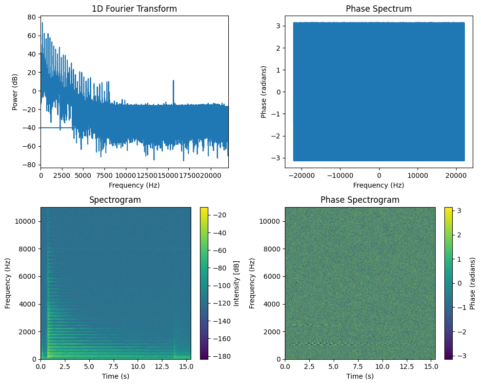
We show above the spectrum of the full audio recording (about 15s) in both magnitude and phase (which is arguably harder to interpret directly). Using a single spectrum to describe the frequency content of a long recording is often innadequate. Over the 15 seconds of recording, there are times when the note is not played or when the timbre changes. High frequencies tend to dissipate faster than low frequencies. Therefore, in audio signal processing, the spectrogram (magnitude and phase) that contains spectra for small time windows is incredibly useful. We see that the magnitude spectrogram of a single note contains rich information. The comb-shaped spectra fades over time, the hammer action is visible at around 0.5s, and some noise occurs at around 12s. The phase spectrogram works similarly and, while it is harder to read, it contains a lot of information. In particular, we can decipher the various partials of the comb. For AMT, we typically use only the magnitude spectrogram and discard the phase spectrogram.
An interesting property of the spectrogram of a single note is that it is well approximated by a rank-one matrix. This suggests using a low-rank model to analyse more complex signals and perform AMT. NMF for AMT, however, has several issues: the rank-one hypothesis is overly strong, the source mixture is non-linear, and there are too few guarantees of uniqueness. I addressed these issues partially in my work on weakly-supervised convolutive NMF for AMT; my contributions are detailed in Automatic Music Transcription.
Music structure estimation#
We can also use spectrograms of full songs to detect similarities between bars. I will not detail this contribution in this manuscript; it was already detailed in length in Axel Marmoret’s PhD manuscript [Marmoret, 2022]. There are also available tutorials in the BarMusComp toolbox link and the more recent Autosimilarity Segmentation toolbox link. The main methodological tool to enhance the similarity detection is the Nonnegative Tucker Factorization of the tensor spectrogram obtained by stacking spectrograms of each bar of a song [Smith and Goto, 2018]. See also the related paragraph in the HDR summary.