
Proco-ALS for fast nCPD#
Reference
[Cohen et al., 2015] J. E. Cohen, R. C. Farias, and P. Comon, “Fast decomposition of large nonnegative tensors,” IEEE Signal Processing Letters, vol. 22, no. 7, pp. 862-866, 2015. pdf
Projected least squares for solving NNLS#
In the NNLS section, we overlooked one possible naive idea for computing an approximate solution: first compute the unconstrained least squares solution, then project it onto the nonnegative orthant. Given a NNLS problem \(\argmin{x\geq 0} \|b - Ax\|_2^2\), the following two lines of code compute this estimate:
    x_hat = tl.solve(A,b)
    x_hat[x_hat<0] = 0
While this solution is not optimal (in fact, there are NNLS instances for which it is arbitrarily far from the solution), it can be much faster to compute, in particular for large and/or structured \(A\) for which highly optimized least squares solvers exist.
A naive algorithm for nonnegative LRA then consists of using this solve-then-project routine as the ALS inner solver. A pitfall to avoid is that sign ambiguity may cause columns of a factor to be all negative at some iteration after the solve operation. Then the projection on the nonnegative orthant yields a zero vector, which makes the next solve ill-posed. A workaround is to flip negative vectors when they occur. The obtained algorithm is coined pro-ALS (projected ALS).
def pro_als_basic(T, r, init, itermax = 100, callback=None):
    # Input tensor T, rank of cp decomposition rank r, init is a cp_tensor
    cp_e = deepcopy(init) # estimated cp_tensor
    norm_tensor = tl.norm(T, 2)
    # compute initial error
    err = tl.norm(T - cp_e.to_tensor(), 2)
    callback(cp_e, err)
    for i in range(itermax): # iterative algorithm loop
        for mode in range(T.ndim): # alternating algorithm loop
            # form MTTKRP, pseudo-inverse and solve least squares
            mttkrp = unfolding_dot_khatri_rao(T, cp_e, mode)
            pseudo_inverse = get_pseudo_inverse(cp_e, r, mode, T)
            factor = tl.transpose(tl.solve(tl.transpose(pseudo_inverse), tl.transpose(mttkrp)))
            # Projection
            # if factor is full negative, flip it
            support = factor<0
            for q in range(r):
                if support[:,q].all():
                    factor[:,q] = -factor[:,q]
                else:
                    factor[:,q][support[:,q]] = 0
            cp_e[1][mode]=factor

        # compute error
        err = err_calc_simple(cp_e,mttkrp,norm_tensor)
        callback(cp_e, err)

    return cp_e, err
We can test this algorithm for computing nonnegative CP on a simple synthetic example.
# Hyperparameters
rank=2
dims = [10,10,10]
# Generate a random CP tensor
np.random.seed(0) # for reproducibility
cp_true = tl.random.random_cp(dims, rank) # rank 2, dim 10x10x10
cp_true[0] = None # no weights
init_cp = tl.random.random_cp(dims, rank)
init_cp[0] = None
for i in range(3):
    cp_true[1][i] = tl.maximum(cp_true[1][i],0)
    init_cp[1][i] = tl.maximum(init_cp[1][i],0)
T = cp_true.to_tensor()
# For error and time tracking
time_0 = time.perf_counter()
times_pro = []
errs_pro = []
def err_ret_pro(_,b):
    errs_pro.append(b)
    times_pro.append(time.perf_counter() - time_0)
# Run pro-ALS
cp_e, err = pro_als_basic(T, rank, init_cp, callback=err_ret_pro)

# Comparison with tensorly nn_cp hals
time_0 = time.perf_counter()
errs_hals = []
times_hals = []
def err_ret_hals(_,b):
    errs_hals.append(b) # returns error unnormalized, convert to error
    times_hals.append(time.perf_counter() - time_0)
# Run HALS ANLS
out2 = non_negative_parafac_hals(T, rank, init=deepcopy(init_cp), callback=err_ret_hals)
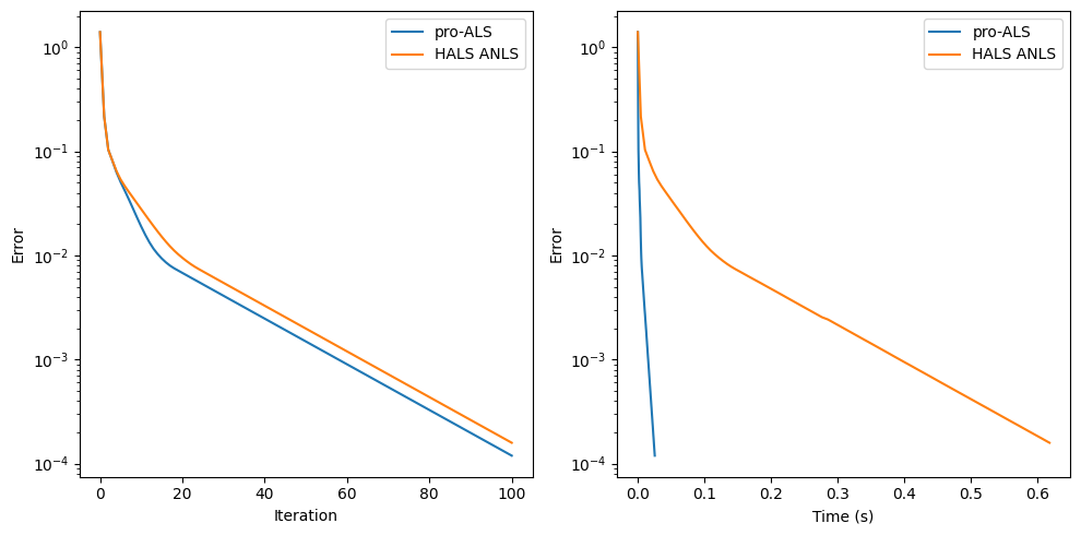
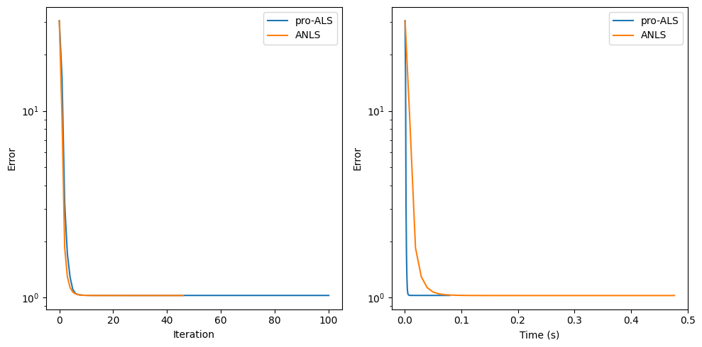
The cost function at each pro-ALS iteration empirically goes down, although this cannot be guaranteed. The algorithm should, in principle, be slower than HALS per iteration, but each iteration is cheap. In practice, for simple problems, it has about the same performance per iteration. For more difficult problems, pro-ALS can, however, struggle to decrease the cost at each iteration. Nevertheless, it performs well on the following realistic example.
from tensorly_hdr.load_eem import load_eem
from tensorly.solvers.penalizations import scale_factors_fro

# Load fluorescence chemometrics data
metadata, noisy_data, clean_data = load_eem()
rank = 3

# Random initialization
np.random.seed(12)  # for reproducibility
init_cp = tl.random.random_cp(clean_data.shape, rank)
init_cp[0] = None
for i in range(3):
    init_cp[1][i] = tl.abs(init_cp[1][i])

# For error and time tracking
time_0 = time.perf_counter()
errs_hals = []
times_hals = []
def err_ret_hals(_,b):
    errs_hals.append(b)
    times_hals.append(time.perf_counter() - time_0)
# Run HALS ANLS
out2 = non_negative_parafac_hals(clean_data, rank, init=deepcopy(init_cp), callback=err_ret_hals)
# Also run pro-ALS
time_0 = time.perf_counter()
errs_pro = []
times_pro = []
def err_ret_pro(_,b):
    errs_pro.append(b)
    times_pro.append(time.perf_counter() - time_0)
# Run pro-ALS
cp_e, err = pro_als_basic(clean_data, rank, init=deepcopy(init_cp), callback=err_ret_pro)
Note on the suboptimality of projected least squares estimates#
Using \(\left[A^\dagger b\right]_+\) as the solution to a NNLS problem \(\min_{x\geq 0} \|Ax - b\|_2^2\) can be a terrible idea for some problem instances. We can use NumPy to generate examples in which projected least squares solutions are arbitrarily far from the true NNLS solutions, even in dimensions two. This may happen in particular when the linear system is poorly conditioned. In the plot below, the projected least squares solution is always zero, but the NNLS solution can be made arbitrarily large by stretching and rotating the mixing matrix \(A\) as desired.
import numpy as np
import matplotlib.pyplot as plt
# Generate data
grid_x = np.meshgrid(np.linspace(-1,1,50),np.linspace(-2,2,50))
grid_z = np.copy(grid_x[0])
theta = 3.14/12
A = np.array([[1,0],[0,0.01]])@np.array([[np.cos(theta), -np.sin(theta)],[np.sin(theta), np.cos(theta)]]) #scale and rotate
x_LS = np.array([-0.5,-0.2])
b = A@x_LS

# LS, Pro-LS, NNLS sols
x_pro_LS = np.maximum(x_LS,0)
x_NNLS = tl.solvers.nnls.active_set_nnls(A.T@b,A.T@A)
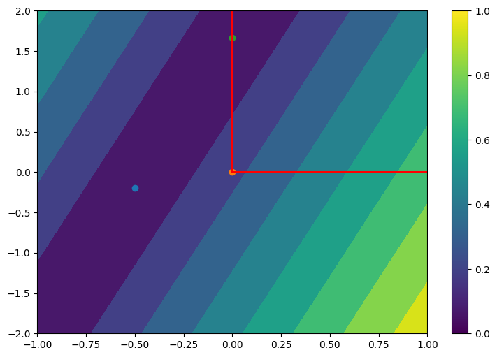
Color stands for the contour lines of the cost \(\|Ax-b\|_2\). Red lines mark the nonnegative orthant. The solution to the LS problem is at the center of the darkest ellipse.
Proco-ALS#
Tucker compression for faster CP-Decomposition#
The true interest of pro-ALS lies in its use in conjunction with Tucker compression. The idea of Tucker compression is to first compute an orthogonal, approximate Tucker decomposition with small inner dimensions using, e.g., HOSVD, then work on the resulting smaller core tensor to compute the CP decomposition.
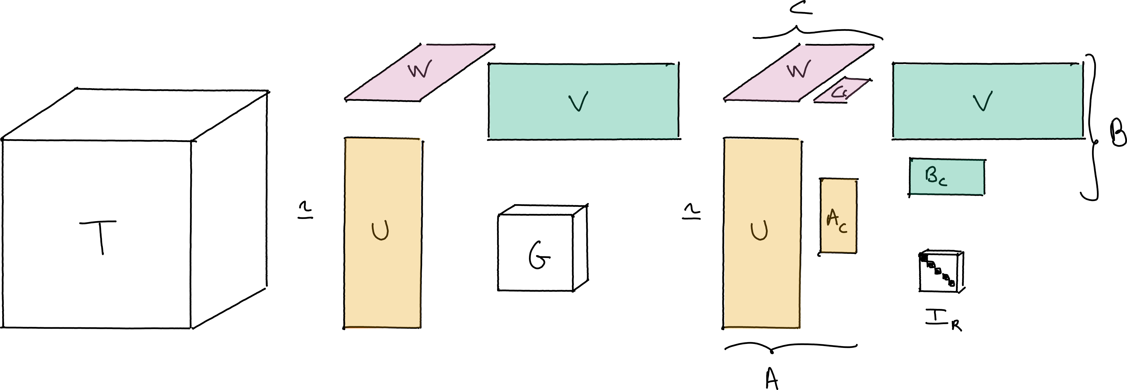
Fig. 28 Illustration of Tucker compression used before the computation of the CP decomposition. The core tensor \(G\) is significantly smaller than the original tensor \(T\), and therefore the CP decomposition of tensor \(G\) is obtained faster than for \(T\). If the Tucker decomposition is accurate and computed efficiently, Tucker compression before CP decomposition can lead to a significant speed-up of the CP decomposition of tensor \(T\).#
Mathematically, this makes sense because of the associativity of the multiway tensor product:
where the tensor \(\left(A_c\otimes B_c\otimes C_c \right) I_r \in \mathbb{R}^{r_1\times r_2\times r_3}\) can be understood as a core tensor \(G\) with a CP decomposition of rank \(r\) and small factors \(A_c,B_c,C_c\).
In tensorly, we can perform Tucker compression (also called CANDELINC [Carroll et al., 1980]) easily as follows
cp_true = tl.random.random_cp([100,100,100], 3)
T = cp_true.to_tensor()

# Perform Tucker on T
t_tensor = tl.decomposition.tucker(T, [3,3,3])
# Perform CP on G
G = t_tensor[0]
small_cp_est = tl.decomposition.parafac(G, 3)
# Recover larger cp by chain rule
cp_est = tl.cp_tensor.CPTensor((small_cp_est[0], [t_tensor[1][i]@small_cp_est[1][i] for i in range(T.ndim)]))

# Comparing with direct cp algorithm
cp_est_direct = tl.decomposition.parafac(T, 3)
Relative reconstruction error of ALS with Tucker compression 0.00022316818891910488
Relative reconstruction error of ALS without Tucker compression 0.00022316818891931621
In this noiseless experiment, Tucker compression is lossless.
Tucker compression for Nonnegative CP#
This procedure is standard for unconstrained CP as it offers little inconvenience when high precision is not required or when the data is noiseless. It is particularly useful when several CP decompositions of the same tensor are to be computed.
However, for nonnegative CP, when working on the core tensor \(G\), one has to keep in mind that nonnegativity applies to the original factors, not the small compressed ones. It means that when updating, e.g., factor \(A_c\) during the CP decomposition of \(G\), the problem to solve is
which is not a typical NNLS problem. It is still a quadratic program; we can solve it up to machine precision with a variety of algorithms. However, these algorithms might be costly. Consider a projected gradient descent algorithm
The cost of the gradient step is low due to Tucker compression, but the cost of the projection onto the positive cone of \(U\) can be consequential if \(U\) is a large matrix (which is exactly the setup we consider for Tucker compression). This projection is in fact exactly a collection of \(n_1\) NNLS problems of dimensions \(r\), with \(n_1\) the dimension in the first mode of the original tensor.
In earlier work [Cohen et al., 2015], we proposed to use the pro-ALS idea to avoid resorting to costly NNLS solvers. This gave birth to the proco-ALS algorithm detailed below. We first solve the least squares problem unconstrained, then project onto the constraint set \( UA_c\geq 0\). As mentioned above, such a projection is also costly. We use a heuristic approximate projection instead,
This projector \(\hat{\Pi}\) is one iteration of alternating projection on convex sets (projection on the nonnegative orthant, and on \(\text{col}(U)\) since \(U\) is a frame). In particular, it is a non-expensive operator. This means that iterating \(\hat{\Pi}\) several times would converge towards \(\Pi_{Ux\geq 0}\). However, for performance reasons, we recommend running it only once.
def proco_als(G, r, init, comp_facs, itermax=100):
    # Input tensor G, rank of cp decomposition rank r, init is a cp_tensor, comp_facs are U,V,W
    cp_e = deepcopy(init) # estimated cp_tensor
    norm_tensor = tl.norm(G)
    err = []
    for i in range(itermax): # iterative algorithm loop
        for mode in range(G.ndim): # alternating algorithm loop
            # form MTTKRP, pseudo-inverse and solve least squares
            mttkrp = unfolding_dot_khatri_rao(G, cp_e, mode)
            pseudo_inverse = get_pseudo_inverse(cp_e, r, mode, G)
            factor = tl.transpose(tl.solve(tl.transpose(pseudo_inverse), tl.transpose(mttkrp)))

            # Projection on UA_c >= 0
            # First decompress
            factor_big = comp_facs[mode]@factor
            # if factor is full negative, flip it, otherwise project
            support = factor_big<0
            for q in range(r):
                if support[:,q].all():
                    factor_big[:,q] = -factor_big[:,q]
                else:
                    factor_big[:,q][support[:,q]] = 0
            # recompress
            factor = comp_facs[mode].T@factor_big
            cp_e[1][mode]=factor

        # compute error in the compressed domain
        err.append(err_calc_simple(cp_e,mttkrp,norm_tensor))

    return cp_e, err
Again we can test this proposed proco-ALS algorithm on a simple synthetic dataset.
cp_true = tl.random.random_cp([100,100,100], 3)
init_cp = tl.random.random_cp([100,100,100], 3)
for i in range(3):
    cp_true[1][i] = tl.maximum(cp_true[1][i],0)
    init_cp[1][i] = tl.maximum(init_cp[1][i],0)
cp_true[0] = None
init_cp[0] = None
T = cp_true.to_tensor()

# Perform Tucker on T
t_tensor = tl.decomposition.tucker(T, [3,3,3])
# Perform CP on G
G = t_tensor[0]
init_small = tl.cp_tensor.CPTensor((None,[t_tensor[1][i].T@init_cp[1][i] for i in range(T.ndim)]))
small_cp_est, err = proco_als(G, 3, init_small, t_tensor[1])
# Recover larger cp by chain rule
cp_est = tl.cp_tensor.CPTensor((small_cp_est[0], [t_tensor[1][i]@small_cp_est[1][i] for i in range(T.ndim)]))

# Comparing with direct cp algorithm
cp_est_direct = tl.decomposition.non_negative_parafac_hals(T, 3)
Relative reconstruction error of ALS with Tucker compression 4.566109437929688e-06
Relative reconstruction error of ALS without Tucker compression 0.17070784831547367
In this example without noise and with perfectly hand-picked multilinear ranks, Tucker compression using proco-ALS helps converging toward the optimal nCP much faster.
Note on the Projection \(\Pi\)
We use the KKT conditions to show that solving
is equivalent to a NNLS problem
This equivalence also has a geometric interpretation: we either project \(-\hat{x}\) on the dual cone of \(U\) (second problem) or find the closest element to \(\hat{x}\) in the intersection of half planes (first problem).
The Lagrangian for the projection problem writes \(L(x,\mu) = \frac{1}{2}\|x - \hat{x} \|_2^2 - \mu^TUx\) which when minimized w.r.t. \(x\) yields \(x^\ast = \hat{x} + U^T\mu^\ast\). The dual problem is therefore formalized as \( \min_{\mu\geq 0} -\frac{1}{2}\|U^T\mu\|_2^2 + \|U^T\mu\|_2^2 + \mu^TU\hat{x}\) which has the same minimizer than \(\min_{z\geq 0} \frac{1}{2} \|U^Tz + \hat{x}\|_2^2\)
To summarize, we may compute the projection \(\Pi_{U\cdot}(y)\) by first solving several small NNLS problems with mixing matrix \(U^T\). This yields \(z\). Then we compute the projection by using the primal-dual relationship \(\Pi_{Ux}(y) = y + U^Tz\).