Median Second-Order-Majorant for faster NNLS

Reference

[Pham et al., 2025] M-Q. Pham, J. E. Cohen, T. Chonavel, “A fast Multiplicative Updates algorithm for Nonnegative Matrix Factorization”, under review at TMLR arxiv reviews

Separable quadratic majorization minimization

In Nonnegative Regressions: NNLS and NNKL, various equivalent formulations of MU have been discussed. There is, however, one more equivalent procedure that leads to MU updates for both Frobenius loss and KL-divergence loss that we leverage in [Pham et al., 2025] to derive more efficient algorithms for NMF (or nonnegative tensor decomposition). This procedure is not limited to matrix and tensor factorizations.

Instead, let us consider the optimization problem

We typically consider convex sets for which the projection is easy and cheap to compute.

\[ \argmin{x\in\mathcal{C}} f(x) \]

where \(f:\mathbb{R}^{n} \mapsto \mathbb{R}_+\) is twice-differentiable, and \(\mathcal{C}\) is a convex set. We also require that the Hessian matrix \(\nabla^2 f(x)\) is nonnegative elementwise.

Since \(f\) is twice differentiable, we consider its truncated Taylor expansion for two vectors \(x,y\) in \(\mathbb{R}^{n}\):

\[ \phi_x(y) = f(x) + \langle \nabla f(x), y-x \rangle + \frac{1}{2}\langle \nabla^2 f(x) (y-x), y-x \rangle, \]

and \(\phi_x(y) \approx f(x)\) when vectors \(y\) and \(x\) are close.

The traditional approach to second-order algorithms, and in particular the Newton method, is to minimize \(\phi_{x^{(k)}}(y)\), denote \(x^{(k+1)}\) the minimizer, and repeat this procedure [Bertsekas, 1999]. While the Newton algorithm features super-linear convergence near a stationary point of \(f\), each iteration is computationally expensive. Moreover, Newton’s method typically does not account for non-smooth constraints. Indeed, without constraints,

\[ \argmin{y\in\mathbb{R}^m} \phi_x(y) = x - [\nabla^2f(x)]^{-1} \nabla f(x), \]

while with constraints, the miniminization of \(\phi\) has no closed form expression. In the particular case where \(\mathcal{C}\) is the nonnegative orthant, minimizing the second-order approximation \(\phi\) amounts to solving an NNLS problem.

More can be read about Newton and quasi-Newton algorithms in [Bertsekas, 1999].

Therefore, significant efforts have been made towards designing simpler algorithms than Newton’s method that still utilise second-order information to some extent. Among others, Gauss-Newton, Levenberg-Marquardt, and LBFGS are popular methods. Maybe the simplest way to change the quadratic estimation of the cost function is to replace the Hessian matrix by a diagonal matrix \(A(x)\),

\[ \psi_x(y) = f(x) + \langle \nabla f(x), y-x \rangle + \frac{1}{2}\langle A(x) (y-x), y-x \rangle. \]

The quadratic function \(\psi_x\) is separable, therefore finding the minimum of \(\psi_x\) is cheap even under the presence of constraints:

\[ \argmin{y\in\mathcal{C}} \psi_x(y) = \argmin{y\in\mathcal{C}} \sum_{i=1}^{n} \nabla f(x)[i] y[i] + \frac{1}{2} A[i,i] (y[i]-x[i])^2 \]

where \(\Pi_{\mathcal{C}}\) denotes the projection on the convex set \(\mathcal{C}\). For many constraint sets, including nonnegativity and cardinality constraints (more generally, for any separable prior, stable by elementwise nonnegative scaling), the solution is given in closed form as

\[ \Pi_{\mathcal{C}} \left( x - \frac{\nabla f(x)}{\text{diag}\left(A(x)\right)} \right). \]

The core design choice is the construction of the diagonal matrix \(A(x)\). Inspired by the proof technique of Lee and Seung for the convergence of MU, we observed with Mai Quyen Pham that for any positive vector \(u\in\mathbb{R}^n\) and for elementwise nonnegative Hessian matrices, any matrix of the form

\[ A_u(x) = \text{Diag}\left(\frac{\nabla^2 f(x) u}{u}\right) \]

For a quadratic loss function \(f\), the SOM algorithm is guaranteed to converge since each iteration decreases the cost. However, this form of convergence is very weak: we only know that the values of the cost function will stagnate asymptotically, but the estimated minimizer need not be the true minimizer. This result can be refined with the SUM framework [Razaviyayn et al., 2013]. Moreover, the convergence rate of SOM in the general case is unknown. In our work, we prove linear convergence of the iterates for the specific problem of NMF with beta-divergence loss.

is a majorant of the Hessian, namely \(A_u(x) - \nabla^2 f\) is semi-definite positive. The proof is straightforward and can be found in [Pham et al., 2025]. If matrix \(A(x)\) is a majorant of the Hessian, we obtain a majorization minimization algorithm as long as \(f\) is a quadratic function, because the truncated second-order Taylor expansion is exact. When \(f\) is not quadratic, the proposed procedure, which, as far as we know, has not been explored in the optimization literature (at least for computing NMF), is coined Second-Order Majorant (SOM), because we minimize a majorant of a separable second-order approximation of the cost function.

MU algorithm as quadratic majorant minimization

The SOM algorithm reduces the design of the diagonal matrix \(A_u(x)\) to choosing a positive vector \(u\). Any choice of \(u\) ensures that \(A_u(x)\) is a majorant of the Hessian and therefore that the obtained algorithm is principled. It turns out that for an NNLS problem, the MU algorithm is a particular case of SOM when \(u=x\). Indeed, for \(f(x) = \frac{1}{2}\|y - Wx\|_2^2\) and nonnegativity constraints, the hessian matrix writes \(\nabla^2 f(x) = W^TW\), and the majorant matrix \(A_u(x)\) with \(u=x\) is

\[ A_x(x) = \text{Diag}\left(\frac{W^TWx}{x}\right). \]

Recall from that this is exactly the diagonal preconditioner that MU utilizes, when understanding MU as a preconditioned gradient descent algorithm. Therefore, setting \(u=x\) yields the MU update with a projection operator

\[ x^{(k+1)} = \Pi_{\mathcal{C}}\left(x^{(k)}\frac{W^Ty}{W^TWx} \right). \]

mSOM: choosing an optimal majorant to the quadratic approximation of \(f\)

Another interesting choice of criterion is the min-max over the diagonal elements of the preconditioner. We show in this work that this is equivalent to Gradient Descent with an optimal stepsize.

The core idea in the joint work with Mai Quyen Pham and Thierry Chonavel [Pham et al., 2025] is to select a vector \(u\) so that \(A_u(x)\) is as small as possible. This amounts to choosing the inverse of the gradient stepsizes as small as possible. We discuss several possible metrics to measure the magnitude of \(A_u(x)\), but one design choice that leads to a closed-form expression is to minimize the median values in \(A_u(x)\), namely

\[ u_{mSOM} = \argmin{u>0}\| \frac{\nabla^2 f(x) u}{u} \|_1. \]

Nonnegativity of the Hessian of the cost at any point is a strong assumption in general, but is satisfied in problems of interest to this manuscript, e.g. for NMF with beta-divergence loss.

It can be shown that when \(\nabla^2 f(x)\) is nonnegative, the solution is in fact trivial:

\[ u_{mSOM} = 1_n, \]

and the resulting algorithm is given by

\[ x^{(k+1)} = \argmin{y\in\mathcal{C}} \sum_{i=1}^{n} \nabla f(x)[i] y[i] + \frac{(y[i]-x[i])^2}{\sum_{j}\nabla^2f(x)[i,j]}. \]

In many particular cases, such as nonnegativity constraints, this update further simplifies to

\[ x^{(k+1)} = \Pi_{\mathcal{C}}\left(x^{(k)} -\frac{\nabla f(x)}{\nabla^2 f(x) 1_n}\right). \]

Because this update rule will be used inside an alternating optimization framework, it can be useful not to minimize the majorant but rather to take a larger step by introducing, for \(\gamma\in[0,2]\), the update

(12)\[ x^{(k+1)} = \Pi_{\mathcal{C}}\left(x^{(k)} -\gamma\frac{\nabla f(x)}{\nabla^2 f(x) 1_n}\right). \]

We call the algorithm with update rule (12) the median SOM algorithm (mSOM). One has to be mindful of a few properties of mSOM:

• for non-quadratic loss functions, it is not guaranteed to decrease the cost function. In fact, mSOM can diverge if initialized poorly. We prove in [Pham et al., 2025] that for \(f(x) = \KL{y, Wx}\) (or any \(\beta\)-divergence with \(\beta\in[1,2[\)) and in the noiseless case, linear convergence happens but is only local. In practice, we observe convergence problems in the first few iterations that can be avoided by using a properly scaled initialization, either by using a few iterations of another algorithm as initialization or by checking numerically that the costs decrease.

• for quadratic loss, the mSOM algorithm is a proper MM algorithm, and we show that it converges linearly globally for any \(\gamma\) in \([0,2]\).

We can visualize the different majorants of the cost (MU majorant, mSOM majorant, and usual gradient descent with optimal stepsize) on a numerical example.

import numpy as np
import matplotlib.pyplot as plt

# Data generation
np.random.seed(0)
[n,m] = [3,4]
W = np.random.rand(m, n)
# worse conditionning makes mSOM and Gradient descent more visibly distinct
W[:,2] = 0.1*W[:,2]+0.45*W[:,0] + 0.45*W[:,1]  # col 3 is col 1 + col 2
xmin = np.random.rand(n)
y = W@xmin

def maj(xk,x,W,y, case='MU'):
    """ Majorant function for the Frobenius NNLS loss at xk, obtained with the MU algorithm.
    returns MU, mSOM and GD majorants
    """
    Wxk = W@xk
    WtW = W.T@W
    Wty = W.T@y
    if case=='MU':
        Precond = WtW@xk/xk
    elif case=='mSOM':
        Precond = WtW@np.ones(n)
    elif case=='GD':
        Precond = np.linalg.norm(WtW, 2)*np.ones(n)
    return np.sum((Wxk - y)**2) + (x - xk).T@(2*WtW@xk - 2*Wty) + np.sum(Precond * (x - xk)**2),


def loss_compute(x0, v, t, W, y):
    """ Compute the Frobenius NNLS loss at x0 + t*v, restricted to the nonnegative orthant.
    """
    steps = [v*t[i] for i in range(len(t))] 
    xs = [x0 + steps[i] for i in range(len(t))]
    return [ [np.linalg.norm(y - W@xs[i])**2 for i in range(len(t)) if np.min(xs[i])>=0],
             [maj(x0, xs[i], W, y, case="MU") for i in range(len(t)) if np.min(xs[i])>=0],
             [maj(x0, xs[i], W, y, case="mSOM") for i in range(len(t)) if np.min(xs[i])>=0],
             [maj(x0, xs[i], W, y, case="GD") for i in range(len(t)) if np.min(xs[i])>=0],
             ], [t[i] for i in range(len(t)) if np.min(xs[i])>=0]

# We plot the Frobenius NNLS loss on three 1d slices of the 3d cost
v1 = np.array([1, 0, 0])
v2 = np.array([0, 1, 0])
v3 = np.array([0, 0, 1])

x0 = xmin + np.array([0.2, 0.5, 0.1])  # we plot the loss centered on this point

t = np.linspace(-1, 0.5, 100)
[L1, Lmu1, LmSOM1, LGD1], ts1 = loss_compute(x0, v1, t, W, y)
[L2, Lmu2, LmSOM2, LGD2], ts2 = loss_compute(x0, v2, t, W, y)
[L3, Lmu3, LmSOM3, LGD3], ts3 = loss_compute(x0, v3, t, W, y)

Show code cell source

Hide code cell source

# Plot the three curves in the same figure with subplots
fig, ax = plt.subplots(1,3, figsize=(8, 4))
ax[0].plot(ts1, L1, label='loss')
ax[0].plot(ts1, Lmu1, label='MU maj')
ax[0].plot(ts1, LmSOM1, label='mSOM maj')
ax[0].plot(ts1, LGD1, label='Lipschitz maj')
ax[0].set_title(f'Loss along {v1}')
ax[0].set_xlabel('increment')
ax[0].set_ylabel('Loss')
ax[0].legend()
ax[1].plot(ts2, L2, label='loss')
ax[1].plot(ts2, Lmu2, label='MU maj')
ax[1].plot(ts2, LmSOM2, label='mSOM maj')
ax[1].plot(ts2, LGD2, label='Lipschitz maj')
ax[1].set_title(f'Loss along {v2}')
ax[1].set_xlabel('increment')
ax[1].set_ylabel('Loss')
ax[1].legend()
ax[2].plot(ts3, L3, label='loss')
ax[2].plot(ts3, Lmu3, label='MU maj')
ax[2].plot(ts3, LmSOM3, label='mSOM maj')
ax[2].plot(ts3, LGD3, label='Lipschitz maj')
ax[2].set_title(f'Loss along {v3}')
ax[2].set_xlabel('increment')
ax[2].set_ylabel('Loss')
ax[2].legend()
plt.tight_layout()
plt.show()

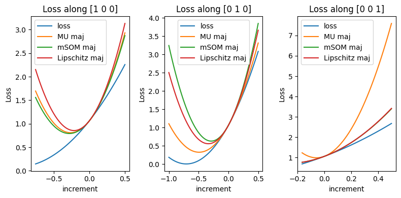
Notice that, in this toy example, while mSOM is designed to be sharper than MU in median along the line \(t[0,1,0]\), MU is tighter.

Alternating mSOM for NMF

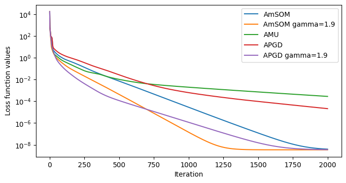
Equipped with the mSOM solver for nonnegative convex problems, one may factorize NMF using an alternating optimization strategy, with mSOM as the inner solver. The following code implements the resulting Alternating mSOM (AmSOM) for NMF with the Frobenius loss and compares it with alternating MU (AMU) and alternating projected Gradient Descent (APGD) on a toy synthetic dataset. The AmSOM updates rules for this problem formalized as \(\argmin{W,H\geq \epsilon} \|Y-WH^T\|_F^2\) are

\[\begin{split} H \leftarrow \max\left(H - \gamma\frac{1}{\mathbb{1}_{n\times r}W^TW}\left(HW^TW - Y^TW \right) , \epsilon \right), \\ W \leftarrow \max\left(W - \gamma\frac{1}{\mathbb{1}_{m\times r}H^TH}\left(WH^TH - YH \right) , \epsilon \right). \end{split}\]

import numpy as np
import matplotlib.pyplot as plt


def mSOM_update(HtH, YH, W, precond, gamma=1.9, epsilon=0):
    ''' Computes the mSOM update rules for the NNLS problem min_{W\geq 0} ||Y - WH^T||_F^2
    '''
    W = np.maximum(W - gamma * precond * (W @ HtH - YH), epsilon) 
    return W

def MU_update(HtH, YH, W, epsilon=0):
    ''' Computes the mSOM update rules for the NNLS problem min_{W\geq 0} ||Y - WH^T||_F^2
    '''
    W = np.maximum(W * (YH / (W @ HtH)), epsilon) 
    return W

def AmSOM(Y, Winit, Hinit, method="mSOM", niter=100, gamma=1.9, epsilon=0):
    ''' Alternating mSOM for the NNLS problem min_{W,H\geq 0} ||Y - WH^T||_F^2
    Using 10 inner iterations for the mSOM updates of W and H.
    '''
    W = np.copy(Winit)
    H = np.copy(Hinit)
    loss = [1/2*np.linalg.norm(Y - W @ H.T, 'fro')**2]
    for it in range(niter):
        HtH = H.T @ H
        if method=="GD":
            step = 1/np.linalg.norm(HtH,2)
        YH = Y @ H
        precond_W = 1/np.sum(HtH, axis=1)  # makes use of broadcasting
        for _i in range(10):
            if method == "MU":
                W = MU_update(HtH, YH, W, epsilon=epsilon)
            elif method=="mSOM":
                W = mSOM_update(HtH, YH, W, precond_W, gamma=gamma, epsilon=epsilon)
            elif method=="GD":
                W = np.maximum(W - gamma*step*(W@HtH - YH), epsilon)

        WtW = W.T @ W
        if method=="GD":
            step = 1/np.linalg.norm(WtW,2)
        YW = Y.T @ W
        precond_H = 1/np.sum(WtW, axis=1)  # makes use of broadcasting
        for _i in range(10):
            if method == "MU":
                H = MU_update(WtW, YW, H, epsilon=epsilon)
            elif method=="mSOM":
                H = mSOM_update(WtW, YW, H, precond_H, gamma=gamma, epsilon=epsilon)
            elif method=="GD":
                H = np.maximum(H - gamma*step*(H@WtW - YW), epsilon)

        loss.append(1/2*np.linalg.norm(Y - W @ H.T, 'fro')**2)
    return W, H, loss

# Exemple usage on a toy dataset
np.random.seed(27)
n, m, r = 100, 80, 5
niter = 2000
Wtrue = np.random.rand(n, r)
Htrue = np.abs(np.random.randn(m, r))
Y = Wtrue @ Htrue.T + 1e-6 * np.random.randn(n, m)

Winit = np.abs(np.random.randn(n, r))
Hinit = np.abs(np.random.randn(m, r))

W, H, err_msom = AmSOM(Y, Winit, Hinit, method="mSOM", niter=niter, gamma=1, epsilon=0)
Wg, Hg, err_msomg = AmSOM(Y, Winit, Hinit, method="mSOM", niter=niter, gamma=1.9, epsilon=0)
W_mu, H_mu, err_mu = AmSOM(Y, Winit, Hinit, method="MU", niter=niter, gamma=1, epsilon=0)
W_gd, H_gd, err_gd = AmSOM(Y, Winit, Hinit, method="GD", niter=niter, gamma=1, epsilon=0)
W_gdg, H_gdg, err_gdg = AmSOM(Y, Winit, Hinit, method="GD", niter=niter, gamma=1.9, epsilon=0)

Show code cell source

Hide code cell source

# comparing the convergence plot
plt.figure(figsize=(8,4))
plt.semilogy(err_msom, label='AmSOM')
plt.semilogy(err_msomg, label='AmSOM gamma=1.9')
plt.semilogy(err_mu, label='AMU')
plt.semilogy(err_gd, label='APGD')
plt.semilogy(err_gdg, label='APGD gamma=1.9')
plt.xlabel('Iteration')
plt.ylabel('Loss function values')
plt.legend()

plt.show()

Other loss functions?

The mSOM framework also applies to NMF with beta-divergences as loss functions. Convergence guarantees are only local, and the empirical results are less significant. Improving mSOM for non-quadratic losses and sparse datasets is a future research direction.