
Multiple dictionaries#
Reference
[Cohen and Gillis, 2018] J. E. Cohen, N. Gillis, “Spectral Unmixing with Multiple Dictionaries”, IEEE Geoscience and Remote Sensing Letters, vol.15 issue 2, pp. 187-191, 2018. pdf
In the one-sparse DLRA section, we have seen that in the context of spectral unmixing, we may use the whole hyperspectral image \(Y\) as a dictionary. Then computing one-sparse DLRA means identifying pure pixels in the image \(Y\) whose spectra correspond to a single material.
While this approach can, in principle, detect pure pixels, the optimisation problem is in fact difficult to solve: the dictionary contains as many atoms as there are pixels, and these atoms are highly correlated. A potential workaround, proposed in [Cohen and Gillis, 2018], is to consider a subset of the image. The user might select regions on a projected view of \(Y\), typically in an RGB visualization, believing they contain pure pixels.
In fact we may go further, and assume that the user selects \(p\) regions \(D_i:=Y_n[:, S_i]\) in the image where \(S_i\) collects the indices of the pixel in the \(i\)th zone from the columnwise \(\ell_2\) normalized image \(Y_n\), and that the user guesses how many pure pixels \(d_i\) are to be found in each zone, at most. Finding the pure pixels in each zone and the corresponding abundances can then be formalized as follows:
where \(\mathcal{K}_i\) is the set of selected pure pixels in the user-defined zone \(S_i\), and \(\#\mathcal{K}\) stands for the number of elements in the set \(\mathcal{K}\), see the illustration below.
import tensorly as tl
from tensorly.datasets import data_imports
import matplotlib.pyplot as plt
import matplotlib.patches as patches
from myst_nb import glue

# Import an hyperspectral image
image_bunch = data_imports.load_indian_pines()
image_t = image_bunch.tensor # x by y by wavelength
image_t = image_t/tl.max(image_t) # maximum value set to 1

# Define zones with pure pixels
# Indian Pines is 145 by 145 (pixels) by 200 (bands)
n1, n2, n3 = tl.shape(image_t)
rank = 5
zx = [[100, 120], [50, 60], [100, 110], [10, 130]]
zy = [[110, 130], [80,90], [15, 25], [4, 90]]
d = [1, 1, 1, 2] # we aim to find 1, 1, 1 and 1 pure pixels in each zone
D = [tl.unfold(image_t[zx[i][0]:zx[i][1], zy[i][0]:zy[i][1], :], 2) for i in range(len(zx))] # unnormalized

# Vectorize the tensor into a n_1\times n_2 matrix (wavelength \times pixels, y vary first)
image = tl.unfold(image_t, 2)


# Show the hyperspectral image at a given band
fig1, ax1 = plt.subplots()
band = 70  # which spectral band to show
ax1.imshow(image_t[:,:,band], cmap="Greys")
colors = ['b', 'y', 'g', 'm', 'r', 'k']
for i in range(len(zx)):
    rect = patches.Rectangle((zx[i][0], zy[i][0]), zx[i][1]-zx[i][0], zy[i][1] - zy[i][0],
                             linewidth=3, edgecolor=colors[i], facecolor='none')
    ax1.add_patch(rect)
plt.close()
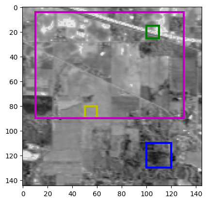
Fig. 25 Showing the hyperspectral image at the 70th band. Colored zones mark the position of the hand-picked pure pixel zones. The dictionaries \(D_i\) have shapes [(200, 400), (200, 100), (200, 100), (200, 10320)]. We seek [1, 1, 1, 2] atoms in each dictionary.#
Solving this multiple-dictionary one-sparse DLRA problem seems daunting. However, it is not much more difficult than solving a one-sparse DLRA if an alternating optimization strategy is used. Solving for matrix \(B\) with fixed pure pixel indices is a simple NNLS. When fixing matrix \(B\), estimating pure pixel indices \(\mathcal{K}_i\) for each dictionary is combinatorial. Nevertheless, we can adapt the MC-ALS strategy to handle this problem:
First, given an estimate for matrix \(B\), compute \( A := \underset{A\geq 0}{\text{argmin}} \|Y - AB^T \|_F^2 \) with a NNLS solver.
Then, fixing \(A\), we find the pure pixel indices by solving the following optimization problem:
This quadratic cost can be turned into a linear cost since the dictionaries are normalized columnwise and all quantities are nonnegative.
where \(\langle A,D\rangle = \text{Tr}(A^TD)\) is the usual scalar product for matrices. This problem can be seen as a linear sum assignment problem, for which efficient solvers are known [Kuhn, 1955]. First, we may assume that all \(d_i\) are equal to one, since we can always duplicate any dictionary \(D_i\) to handle \(d_i>1\). When \(d_i=1\) for all \(i\leq p\), for each dictionary \(D_i\), only one atom can be selected. It is therefore natural to define a distance between a column \(j\) of matrix \(A\) and the whole dictionary \(D_i\), here stored in a matrix \(C\in\mathbb{R}^{p\times r}\)
Then the problem of finding pure pixels with the precomputed matrix \(A\) boils down to solving
where \(\mathcal{P}(p,r)\) is the set of surjective permutations from \([1,p]\) to \([1,r]\). This is a classical formulation of the linear sum assignment problem (with \(p\) possibly larger than \(r\)).
Note
Building on top of the above derivation, we may in fact use any reasonable distance between atoms in dictionaries \(D_{i}\) and columns of \(A\) to compute a cost matrix \(C\), such as the Spectral Angular Mapper [Boardman, 1993, Kruse et al., 1993]. The MC-ALS is a heuristic; in particular, the choice of this distance need not be driven by the noise model for the data \(Y\).
We may implement the resulting Multiple dictionaries MC-ALS (M2C-ALS) similarly to MC-ALS. Below is the algorithm for estimating the pure pixels. We will assume nonnegativity is always satisfied by the data and estimated parameters.
from scipy.optimize import linear_sum_assignment
import tensorly as tl
import numpy as np

def M2C_ALS_Aestimation(Y, D, B, d, A0=None):
    # D = [D_1, ..., D_p] is a list of normalized dictionaries
    # d = [d_1, ..., d_p] is the list containing the bounds on the number of pure pixels

    if A0 is None:
        Ahat = tl.solvers.hals_nnls(B.T@(Y.T), B.T@B, n_iter_max=20).T
    else:
        Ahat = tl.solvers.hals_nnls(B.T@(Y.T), B.T@B, n_iter_max=20, V=A0.T).T
    Ahatn = Ahat/tl.norm(Ahat, axis=0)
    n, r = tl.shape(Ahat)

    p = sum(d)
    C = tl.zeros([p, r])
    best_atoms_i = tl.zeros([sum(d), r], dtype=int)
    best_atoms_idx = tl.zeros([sum(d), r], dtype=int)

    # Compute the distances between dictionaries D_i and columns of A, duplicating when d_i>1
    # Keep in memory the position of the atoms in the dictionaries that maximize the distance
    idx_1 = 0
    for i in range(len(d)):
        idx_0 = idx_1
        idx_1 = idx_1+d[i]
        cross_product = D[i].T@Ahatn
        for j in range(r):
            idx_max = tl.argmax(cross_product[:,j])
            C[idx_0:idx_1, j] = cross_product[idx_max, j]
            best_atoms_i[idx_0:idx_1, j] = i
            best_atoms_idx[idx_0:idx_1, j] = idx_max

    # solve the linear assignement problem
    K, _ = linear_sum_assignment(C, maximize=True)

    # Recover the atoms in each dictionary to fill in A
    Ahat2 = tl.copy(Ahat)
    Kis = []
    for ik, k in enumerate(K[:r]):
        i = best_atoms_i[k, ik]
        idx_max = best_atoms_idx[k, ik]
        Ahat2[:, ik] = D[i][:, idx_max]
        # store the atoms in the order they appear in A
        Kis.append((i, idx_max))
    return Kis, Ahat2, Ahat
For a proof of concept of this sub-algorithm, we provide random abundances and select pure pixels in the zones.
# normalize dictionaries and pick random pixels
pix = []
atom_list = []
for i in range(len(D)):
    D[i] = D[i]/tl.norm(D[i], axis=0)
    [pix.append(np.random.randint(D[i].shape[1])) for j in range(d[i])]
    [atom_list.append(D[i][:, pix[-j-1]]) for j in range(d[i])]

A0 = tl.tensor(atom_list).T
B = np.random.rand(n1*n2, rank) #tl.solvers.hals_nnls(A0.T@image, A0.T@A0).T
image_toy = A0@B.T
out = M2C_ALS_Aestimation(image_toy, D, B, d)
The true selected pixels are [350, 21, 78, 5718, 767] (indices are local for each dictionary \(D_i\)). The ones provided by the algorithm, without hints, are [np.int64(350), np.int64(21), np.int64(78), np.int64(767), np.int64(5718)]. Now we can test the full alternating algorithm on Indian Pines and see what it gives, when compared to naive separable NMF such as one-sparse DLRA or SNPA.
def M2C_ALS(Y, D, B_0, d, itermax=100, verbose=False):
    errs = []
    B = np.copy(B_0)
    A = None
    for it in range(itermax):
        # estimate A
        K, A, _ = M2C_ALS_Aestimation(Y, D, B, d, A0=A)
        if verbose:
            print(f"At iteration {it}, the pure pixel indices in each dictionary are {K}")
        # estimate B
        B = tl.solvers.hals_nnls(A.T@Y, A.T@A, n_iter_max=20).T
        # compute error
        errs.append(tl.norm(Y - A@B.T)**2/tl.prod(Y.shape))
        # stop if error has not changed at all (algorithm is stuck)
        if it>1 and errs[-2]==errs[-1]:
            print("Final estimated indices", K)
            print("MSE", errs[-1])
            break
    return (None, [A, B]), errs, K

B0 = np.eye(*B.shape)
#B0 = np.random.rand(*B.shape)  #TODO better init
ABest, errs, Ke = M2C_ALS(image, D, B0, d)
Final estimated indices [(np.int64(0), np.int64(119)), (np.int64(1), np.int64(13)), (np.int64(2), np.int64(64)), (np.int64(3), np.int64(2150)), (np.int64(3), np.int64(2289))]
MSE 0.0002204785844333469
It may be noted that very few iterations are performed in practice; the algorithm gets stuck in a local minimum because of the discrete-continuous nature of the optimization problem. This problem is inherited from the MC-ALS algorithm. Nevertheless, the residuals are rather small, and we have found good candidates for pure pixels within each dictionary \(D_i\). Below, we plot the obtained spectra and abundances, along with their positions within the entire image. We compare with a classical separable NMF approach, SNPA [Gillis and Vavasis, 2014].
# Compare with SNPA
from tensorly_hdr import sep_nmf
from tensorly_hdr.image_utils import convert_to_pixel, convert_to_pixel_from_patches, convert_to_index
Ksep, Asep, Bsep = sep_nmf.snpa(image, rank)
Kxsep, Kysep = convert_to_pixel(Ksep, image_t.shape[1])
# Permute pairs of estimated matrices for better visualisation; also permute the Ksep
# TODO

# Converting estimated indices from M2C-ALS to pixel indices, and vectorized indices
Kx, Ky = convert_to_pixel_from_patches(Ke, zx, zy)
Kee = convert_to_index(Kx, Ky, image_t.shape[1])

print("Selected Pure Pixels based on separable NMF", Ksep)
print("Selected Pure Pixels based on Multiple-Dictionary NMF", Kee)
Selected Pure Pixels based on separable NMF [13225, 19579, 17966, 259, 2516]
Selected Pure Pixels based on Multiple-Dictionary NMF [np.int64(16794), np.int64(11798), np.int64(3149), np.int64(3165), np.int64(3354)]
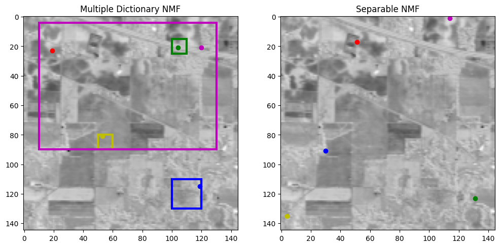
Fig. 26 Selected pure pixels from separable NMF (right) and multiple dictionaries (left). Notice that the pure pixels are located in the user-defined areas with the multiple dictionaries model.#
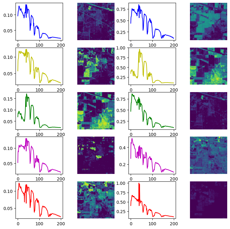
Fig. 27 Estimated spectra and abundance maps from separable NMF (right) and multiple dictionaries M2C-ALS (left)#