Single-pixel hyperspectral image reconstruction and unmixing#
Reference
[Hariga et al., 2024] S. Hariga, J. E. Cohen and N. Ducros, “Joint Reconstruction and Spectral Unmixing from Single-Pixel Acquisitions”, EUPSICO 2024. hal
[Hariga et al., 2025] S. Hariga, A. Repetti, N. Ducros, J. E. Cohen, “Approche plug-and-play pour la reconstruction des cartes d’abondance en imagerie hyperspectrale mono-pixel” GRETSI 2025 hal
[Ducros, 2024] N. Ducros, J. E. Cohen, L. Mahieu-Williame, “Freeform Hadamard imaging: Back to the roots of computational optics”, under review, hal
Single-pixel hyperspectral imaging principle#
Spectral cameras are invaluable tools for acquiring detailed spectral information. They function by spatially spreading an incoming light flux across its constituent wavelengths. This spectral-spatial (Fourier) transformation implies that, by design, it is difficult to acquire spectral images with high spatial and spectral resolution. This is particularly true if the imaging device must remain affordable and lightweight.
Although the idea of compressive acquisitions in computational optics precedes the development of compressive sensing [Nelson and Fredman, 1970], Duarte and co-authors proposed the single-pixel camera for Single-Pixel Imaging (SPI), which uses spatial multiplexing to feed focalized masked images into a high-resolution point spectrometer [Duarte and Baraniuk, 2012, Duarte et al., 2008]. In the setup available at CREATIS, the compressed light flux is the input of a spectrometer. The hyperspectral cube containing both the spatial information (images) and the spectral information (spectra) is then reconstructed by solving an inverse problem, following a long tradition of reconstruction imaging techniques in the computational imaging community [Beneti Martins et al., 2023].
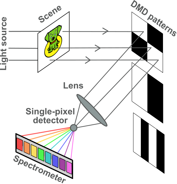
Fig. 36 Representation of the single-pixel camera [credits: Séréna Hariga].#
Let us formalize the problem. Let \(Y\in\mathbb{R}_+^{m\times p}\) be the acquired matrix, with \(m\) the number of measurements or patterns, and \(p\) the number of spectral bands measured by the spectrometer. Each acquisition, say the \(k\)-th, is obtained by summing the pixels of a masked image \(a_k \ast_{1,2} X_t\) where \(a_k\in\{0,1\}^{n_1\times n_2}\) is a binary mask and \(X_t\in\mathbb{R}_+^{n_1\times n_2\times p}\) is the unknown hypespectral cube to reconstruct, with \(n_1\times n_2\) pixels. The elementwise product \(\ast_{1,2}\) indicates that the mask is applied on each slice \(X_t[:,:,i]\) of the hypercube. It can be convenient to vectorize the spatial dimension and consider the vector patterns \(A[k,:]\in\{0,1\}^{n_1n_2}\) as well as the unknown matrix \(X\in\mathbb{R}_+^{n_1n_2\times p}\). The noiseless acquisition is therefore modeled linearly as \(Y = AX\).
The noise model for single-pixel imagers is standardized as a Poisson-Gaussian mixture, see the EMVA Standard 1288. For the sake of simplicity, and since Gaussian noise is typically weak in these acquisitions, we consider the noise to be pure Poisson. Poisson noise arises because the spectrometer counts photons hitting its electronic sensors, and counting errors/fluctuations are well modeled by the Poisson distribution. The model then writes
where \(\alpha\) is the average photon count that can be interpreted as the signal strength. The signal to noise ratio can be shown to be proportional to \(\sqrt{\alpha}\): the higher \(\alpha\) the less noisy the acquisition. We consider that the hypercube \(X\) has normalized intensities in \([0,1]\).
The reconstruction of the hypercube \(X\), knowing the measurements \(Y\) and the acquisition matrix \(A\), is an inverse problem. It is ill-posed in the sense that infinitely many measurements are required to obtain a perfect reconstruction, because of Poisson noise. Furthermore, if the number of patterns is strictly smaller than the number of pixels \(n:=n_1n_2\), the linear system \(Y=AX\) has infinitely many solutions. For both these reasons, regularization is essential in single-pixel image reconstruction. The classical approach is to reconstruct each slice of the hypercube separately, wavelength by wavelength, using state-of-the-art image reconstruction algorithms and priors. In the PhD thesis of Serena Hariga, co-supervised with Nicolas Ducros, we have studied the joint reconstruction and unmixing of the hypercube using spectral regularization [Hariga et al., 2024], as well as spectral unmixing directly from the measurements with spatial priors [Hariga et al., 2025].
Reconstruction wavelength by wavelength (existing work)#
Hadamard patterns#
Before considering a baseline reconstruction method, it is necessary to discuss more about the choice of the acquisition matrix \(A\). There are both practical and theoretical constraints that guide the choice of \(A\).
Practically, the patterns are applied to the image by leveraging a micromirror matrix (DMD). The image is focused on the DMD, which has small mirrors corresponding to pixels that can point in two different directions. All the mirrors that point towards the lens that targets the spectrometer reflect light from the observed object and contribute to the measured spectrum. The mirrors pointing in the opposite direction effectively block the incoming light. Therefore, we may assume that the observation matrix is binary. Contrary to other imaging modalities, such as magnetic resonance imaging, the patterns can be changed at will for each acquisition.
Theoretically, if the patterns could be negative in \([-1, 1]\), the “optimal” acquisition patterns are known to be Hadamard matrices [Nelson and Fredman, 1970]. Optimality here is meant in the sense of statistical minimal linear reconstruction error, i.e., minimal estimation variance. In particular, Hadamard patterns are shown to outperform raster scan, which observes each pixel individually and therefore does not perform spatial multiplexing. The theoretical gain of Hadamard matrices versus raster scan is known as the Felgett advantage.
Why are Hadamard patterns “optimal”
In 1970, Nelson and Fredman introduced the concept of Hadamard spectrocopy [Nelson and Fredman, 1970]. In their seminal work, they prove that Hadamard patterns are an “optimal” choice for the acquisition basis. Let us clarify in what sense this optimality is meant, and under which assumptions.
Nelson and Fredman are concerned with linear reconstructions of acquisitions \(y=Ax + e\), where matrix \(A\) is either the identity matrix (raster scan) or a complete Hadamard basis. The noise \(e\) is supposed to be additive, i.i.d. with finite variance \(\sigma\), but the distribution of \(e\) is not necessarily Gaussian.
Linear reconstructions are of the form \(\hat{x} = By\) with matrix \(B\) defined as the pseudo-inverse of matrix \(A\). This choice for the reconstruction corresponds to the least squares estimation of the unknown \(x\); it is the MLE under Gaussian noise. If the noise is not Gaussian, its statistical meaning is more ambiguous.
The quantity that Nelson and Fredman consider for measuring the quality of the reconstruction is the Root Mean Square Error (RMSE), defined as
RMSE is exactly the average estimation error in \(\ell_2\) norm, and therefore is a reasonable error metric for Gaussian noise. Because matrix \(B\) is the pseudo-inverse of the acquisition operator \(A\), we see that the residual \(x - \hat{x}\) amounts to exactly \(Be\), a centered noise with covariance \(B^TB\) (\(\hat{x}\) is an unbiaised estimate). The RMSE is thus easily derived as
or for the \(i\)-th measurement only,
The Felgett advantage is obtained when comparing the RMSE of Hadamard patterns and raster scan. The ratio of the RMSE\(_i\) values, denoted by \(F_i\), is simply
For raster scan the rows of matrix \(B\) have unit \(\ell_2\) norm, while for Hadamard patterns the rows of \(B=\frac{1}{n}A^T\) have constant norm, \(\sqrt{n}\), which leads to
A reasonable question is whether there exist better choices than Hadamard matrices for maximizing this ratio. Interestingly, Nelson and Fredman show that the ratio \(F\) is bounded by \(\sqrt{n}\). Indeed, by the Cauchy-Schwarz inequality,
Therefore, it holds that \(F_i\leq \|A[i,:]\|_2 \leq \sqrt{n}\) where the last inequality assumes that the measurement operator \(A\) has all values between \(-1\) and \(1\). Hadamard matrices are thus MSE-optimal.
The optimality of the Hadamard patterns, however, is meant under many unrealistic assumptions:
The measurement operator \(A\) has values in \([-1,1]\). The bound on the magnitude is reasonable for SPI, but a DMD can only implement nonnegative entries. Neslon and Fredman discussed this issue and introduced binary \(S\)-matrices, which have a Felgett advantage of \(\frac{n+1}{2\sqrt{n}}\), therefore quasi-optimal.
The noise is additive. In SPI, the noise model is Poisson-Gaussian, so additivity is not a valid assumption.
The reconstruction is linear. Most state-of-the-art reconstruction algorithms employ more sophisticated reconstruction strategies.
The error is measured with the RMSE, which is not a robust or statistically meaningful error metric for Poisson-Gaussian noise.
There are, therefore, ample research avenues for improving upon the (nonnegative) Hadamard patterns design. Revisiting the acquisition patterns, MSE gains for Poisson-Gaussian noise and statistical estimators is one of my research perspectives.
A practical solution for implementing the Hadamard patterns on the DMD is to acquire the positive and negative parts sequentially and concatenate the measurements into a single vector. If the image has \(n\) pixels and \(n\) Hadamard patterns to be acquired, the number of measurements is then \(m:=2n-1\) (one pattern is full of zeros and ignored), and the data vector \(y\) has size \(m\). Doing so preserves the Poisson distribution. Another usual post-processing method computes the difference of the positive and negative acquisitions, resulting in a simulated Hadamard acquisition, but the noise distribution is modified. Formally, we define
where \(H\) here denotes a Hadamard matrix, and \([x]^- \geq 0\) is the negative part of a vector or matrix \(x\). Matrix \([H]^-\) contains a row of zeros that is usually removed.

Fig. 37 Examples of Hadamard patterns stored in the rows of matrix \(H\). Ones are shown in white, and minus ones (zeros in practice) in black. The patterns are orthogonal and have the same number of black and white pixels, except the first two (all white, all black).#
In short, we suppose that measurements \(Y\) are stored in a matrix of size \(m\times p\), and assume the model \(Y\sim \mathcal{P}\left(\alpha AX\right)\) with \(A\) of size \(m\times n\) a matrix with entries in \(\{0,1\}\).
Hadamard matrices have both a simple form for the pseudo-inverse and a cheap matrix-vector product [Magoarou and Gribonval, 2015]. It is natural to question whether one can apply, and invert, the split operator \(A\) at a similar cost, and we show here that both operations can be performed efficiently when \(A\) is the split Hadamard matrix.
First, the product \(A^Ty\) can be obtained using the fast Hadamard transform. Indeed, \([H]^{\pm} = \frac{1}{2} \left[H \pm 1\right]\). Second, the pseudo-inverse \(A^{\dagger}\) admits a closed-form expression, see section 3.5.4 in [Harwit and Sloane, 1979].
where \(1_{n,n}\) is a matrix of ones, and its contraction is implemented as a summation. This is obtained by noting that
and that \( \left( I_n - \frac{1}{n+1}1_{n\times n} \right)\left( I_n +1_{n\times n} \right) = I_n \).
Inversion of the positive Hadamard matrix
Most matrices obtained from the Hadamard matrix admit fast inversion algorithms. The methodology, exemplified on matrix \([H]^+\), is as follows.
Matrix \([H]^+\) is left-invertible, and by noticing that
we get that for any vector \(x\in\mathbb{R}^{n}\),
and vector \(x\) is recovered as
We see that the pseudo-inverse of \([H]^+\) is computed as
which can be efficiently contracted with any vector \(x\) given a fast Hadamard transform algorithm.
We can easily simulate the acquisition with the help of the Python package spyrit, developed at CREATIS [Abascal et al., 2025].
import torch, torchvision
from spyrit.core.meas import HadamSplit2d
from spyrit.core.noise import Poisson
import matplotlib.pyplot as plt
import tensorly as tl
tl.set_backend("pytorch")
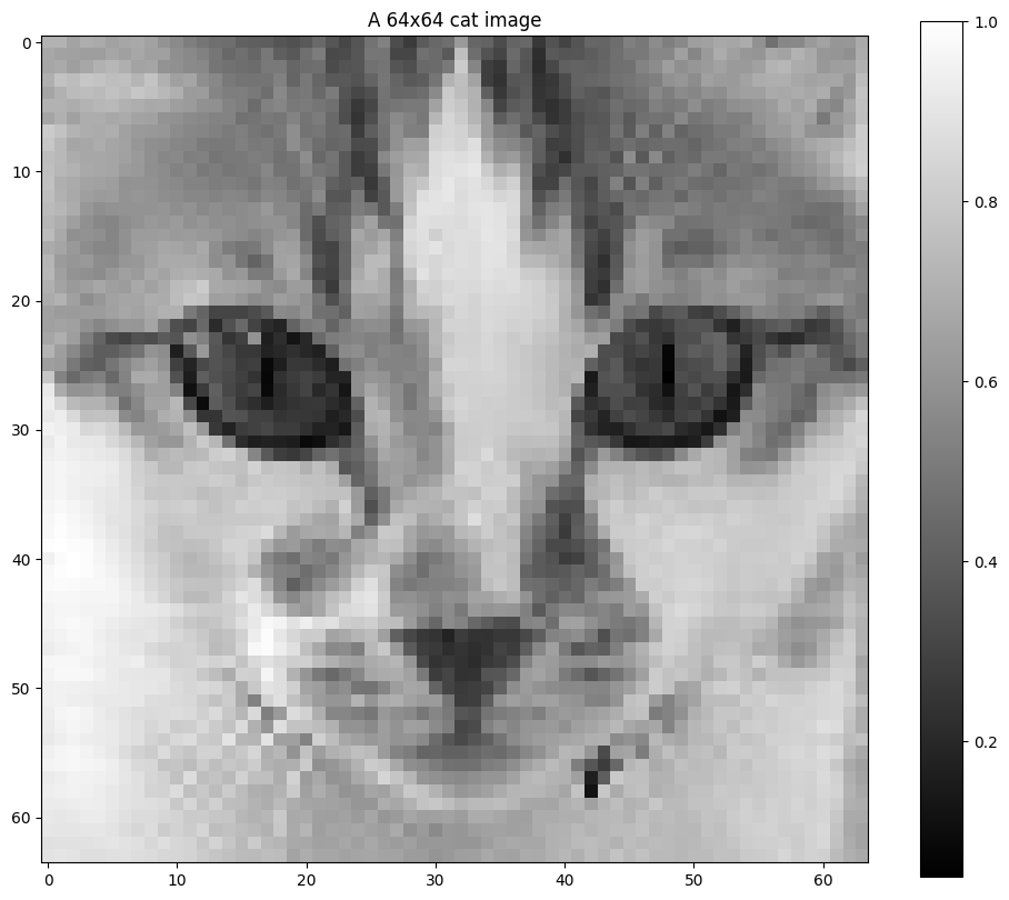
# Cat obtained from https://www.kaggle.com/datasets/mahmudulhaqueshawon/cat-image (small)
x = torch.sum(torchvision.io.read_image("../../tensorly_hdr/dataset/cat.jpg"), axis=0)
x = x/torch.max(x) # normalize to [0,1], this is realistic
plt.figure(figsize=(12,10))
plt.imshow(x, cmap='gray')
plt.colorbar()
plt.title("A 64x64 cat image")
plt.show()
We define the measurement operator and the noise model, then use fast transforms to efficiently simulate the acquisition. Note that while the mathematical discussion in this section is focused on 1D vectors \(x\), SPI involves 2D monochromatic images (or 3D hyperspectral cubes when spectra are considered). The Hadamard and split Hadamard operators can be defined in 2D using separability.
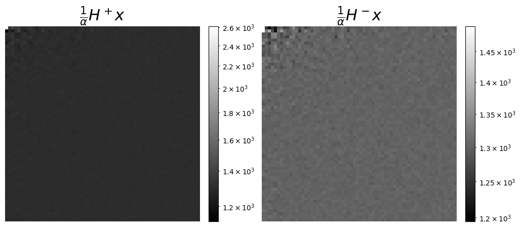
We can also visualize the measurements as coefficients in the Hadamard basis, which can be seen as a wavelet transform. This is more meaningful here to display the coefficients corresponding to the split acquisitions, \([H]^+\) and \([H]^-\).
from matplotlib.colors import LogNorm

alpha=1e2
meas_op = HadamSplit2d(64, noise_model=Poisson(alpha))  # this creates the split measurement operator A, and defines the model parameters (noise level)
y = meas_op.forward(x)  # This sampled y~P(\alpha Ax)
y = y/alpha  # rescale to get back the right intensity scale
print(f"We can check that the shape of y, {y.shape[0]}, is 64^2*2=8192, as expected for a split Hadamard of size 64x64, where the row of zero in A is not removed")

y_pos = y[0::2]
y_neg = y[1::2]  # Note: y[1] is zero

f, axs = plt.subplots(1, 2, figsize=(12, 5))
# increase fontsize of the title
axs[0].set_title(r"$\frac{1}{\alpha}H^+x$", fontsize=22)
# In logscale to better see small values
im = axs[0].imshow(y_pos.reshape(64, 64), cmap="gray", norm=LogNorm())
# add a colorbar, that fits the size of the image, and with fixed range
plt.colorbar(im, ax=axs[0], fraction=0.046, pad=0.04)
axs[1].set_title(r"$\frac{1}{\alpha}H^-x$", fontsize=22)
im = axs[1].imshow(y_neg.reshape(64, 64), cmap="gray", norm=LogNorm())
plt.colorbar(im, ax=axs[1], fraction=0.046, pad=0.04)
# remove axis for the both plots
axs[0].axis('off')
axs[1].axis('off')
plt.show()
We can check that the shape of y, 8192, is 64^2*2=8192, as expected for a split Hadamard of size 64x64, where the row of zero in A is not removed
Reconstruction#
As long as the spectral dimension is ignored and reconstruction, that is, recovering the true image \(x\) from the measurements \(y\), is computed wavelength by wavelength, there are a variety of well-known available methods that are listed thereafter.
Pseudo-inverse reconstruction#
The simplest reconstruction algorithm performs a least squares reconstruction,
This reconstruction has several advantages.
It is unbiased.
It is reasonably cheap to perform as long as the observation matrix \(A\) is not too large. Recall that the pseudo-inverse of matrix \(A\) is known in closed form, and its contraction with a vector or matrix leverages fast Hadamard transforms.
In practice, the spyrit package that we rely on does not yet implement these fast transforms for the split Hadamard measurements without further processing, so the pseudo-inverse computation is quite slow. The solvers I use are not compatible with fast Hadamard transforms and are also quite slow. Since the image is nonnegative, we can also use a NNLS solver such as HALS.
# Reconstruction with pseudo-inverse
x_rec = torch.linalg.lstsq(meas_op.A, y).solution.reshape(64, 64)
print(f"The pseudo-inverse reconstruction has {torch.sum(x_rec<0)} negative entries")
# Bonus: we can use a nnls solver, also very slow without fast operators
from tensorly.solvers.nnls import hals_nnls
Aty = meas_op.adjoint(y)[:,None]
AtA = meas_op.A.T@meas_op.A
x_rec_nnls = hals_nnls(Aty, AtA, n_iter_max=20, tol=0).reshape(64, 64)
The pseudo-inverse reconstruction has 6 negative entries
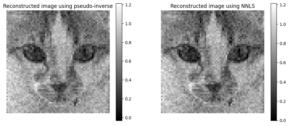
Note that the pseudo-inverse reconstruction gives essentially the same result as the NNLS solver. The two reconstructions are not the same, however, if we did not have to split the acquisitions and could acquire \(Hx\) directly, then they would be the same. Indeed, \(H\) is an invertible matrix and therefore \(x^\ast=H^Ty\) minimizes the loss \(\|y - Hx\|_2^2\). The same solution would also minimize any positive loss \(g(x)\) equal to zero at \(x^\ast\), which includes the MLE discussed next. This observation suggests that the choice of reconstruction method may not significantly affect the results, and that the pseudo-inverse is a good compromise among speed, simplicity, and performance.
We can also show the error map for the pseudo-inverse reconstruction, to observe that the residual is not evidently spatially correlated, despite the misfit between the noise model and the reconstruction loss.
plt.figure(figsize=(12,10))
plt.imshow(torch.abs(x - x_rec), cmap='gray')
plt.colorbar()
plt.axis('off')
plt.title("Error map for pseudo-inverse")
plt.show()
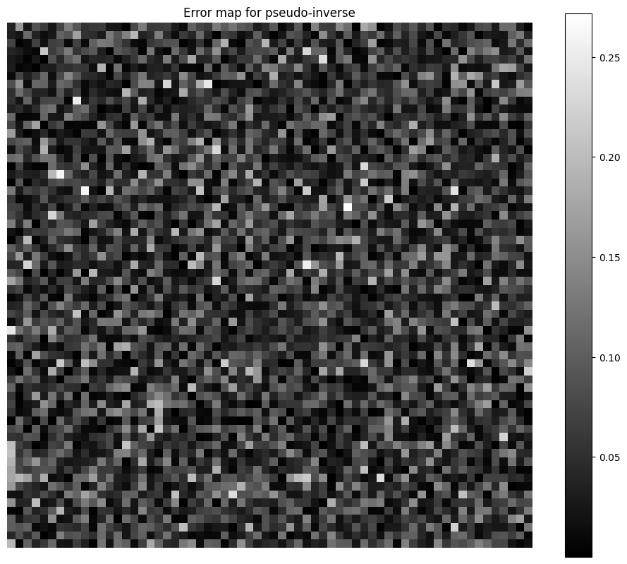
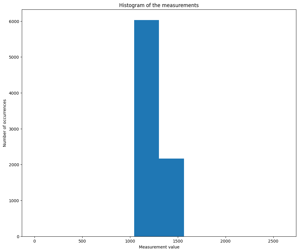
The good performance of the least squares estimate for this Poisson noise problem can be explained by the fact that entries of \(\alpha Ax\) are large and concentrated around the same value \(\frac{1}{2}\alpha \sum_{i\leq n}x[i]\). Indeed, except for the first row of \(A\) and the row of zeros, all rows have exactly half their values set to 1, and the other half to zero. The measurements are therefore essentially bootstraped mean evaluations of the image. This has two consequences:
The empirical measurements \(y_i\) are large enough to obtain a faithful approximation of the (elementwise) Poisson distributions by Gaussian distributions of mean \(\alpha A[i,:]x\) and variance \(\alpha A[i,:]x\).
The variance is essentially the same for all measurements, except \(y[0]\) (corresponding to the row of ones) and \(y[1]\) (corresponding to the row of zeros, and that could be ignored). We denote \(\sigma=\frac{1}{2}\alpha \sum_{i\leq n}x[i]\) the empirical variance estimation. If we consider the model \(y \sim \mathcal{N}(\alpha Ax, \sigma)\), which according to the previous point, should correctly approximate the Poisson distribution, then the pseudo-inverse is a reasonable approximation of the MLE of the image. For Gaussian problems, it is known that the residuals are uncorrelated with the image, this can be observed numerically on the previous example. Below we plot the histogram of the values in the measurement \(y\), to check that they are indeed concentrated around the same numerical value.
Maximum Likelihood reconstruction#
The MLE for Poisson noise is given by the minimizer of the KL-divergence
which can be approximately computed using, e.g., the MU algorithm. Below is an example of MLE reconstruction.
# Reco avec MU
from tensorly_hdr.nmf_kl import Lee_Seung_KL_regression
# remove the second element in y and the row of zeros to avoid division by zero
yr = torch.cat([y[0:1], y[2:]])
Ar = torch.cat([meas_op.A[0:1,:], meas_op.A[2:,:]], dim=0)
crit, x_mu, time, _ = Lee_Seung_KL_regression(yr, Ar, Hini=x_rec_nnls.reshape(64**2), epsilon=1e-8, NbIter=60, tol=1e-6, verbose=True, print_it=20)
------Lee_Sung_KL running------
Loss at initialization: 20.782882690429688
Loss at iteration 1: 20.779123306274414
Loss at iteration 21: 20.77887725830078
Loss at iteration 41: 20.77863311767578
Loss at iteration 60: 20.778409957885742
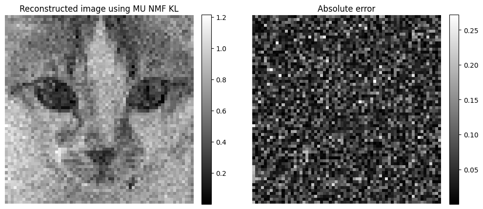
Arguably, in this context, the complication induced by using the Poisson MLE instead of the pseudo-inverse may not be worth the gain in estimation performance. However, the MLE can be easily generalized to measurements that are not Hadamard-based, such as a raster scan that acquires each pixel sequentially. We therefore work with this estimator in the following, with least squares initialization.
Both the least squares and the MLE reconstruction are computed in parallel across wavelengths. Therefore, it is expected that incoherent reconstruction artifacts will be found in the reconstructed spectra. The goal of the works presented subsequently is to use known spectra or spectral priors to improve spectral reconstruction.
Undersampled reconstruction#
The acquisition of the data matrix \(Y\) is performed in parallel along the wavelength dimension, but sequentially along the spatial dimension: Hadamard patterns are loaded onto the DMD one after the other. Each acquisition lasts for a pre-determined time \(\Delta t\); the higher \(\Delta t\), the more signal is acquired. Therefore, to reduce the total acquisition time, one may either reduce \(\Delta t\), which increases the noise level for all acquisitions, or acquire only a subset of the Hadamard patterns. This second choice allows for the acquisition of the most important patterns with a good signal-to-noise ratio. However, the reconstruction using the left pseudo-inverse is no longer available.
One may use the right pseudo-inverse instead of the left one, which is known to amount to solving a problem of the form
Prior information about the image is typically incorporated into the model to ensure identifiability. Classical priors include nonnegativity, sparsity in wavelet bases and sparsity in finite differences, also called Total Variation.
Denoting \(g(X)\) the negative log-prior, reconstruction in the Maximum A Posteriori (MAP) sense is then performed by minimizing
while the regularized least squares estimator is obtained by minimizing
We can illustrate the reconstruction by right pseudo-inverse and the effect of the nonnegativity prior with an NNLS solver, in which case \(g(X)\) is the characteristic function of the nonnegative orthant.
# NNLS with subsampling
yr = torch.cat([y[0:1], y[2:]])
Ar = torch.cat([meas_op.A[0:1,:], meas_op.A[2:,:]], dim=0)
# Removing the second half of measurements
yr = yr[:len(Aty)//2]
Ar = Ar[:len(AtA)//2, :]
# Right pseudo-inverse
x_rec_ls_sub = torch.linalg.pinv(Ar)@yr
x_rec_ls_sub = x_rec_ls_sub.reshape(64,64)
# MU initialized with the pseudo-inverse
crit, x_mu_sub, time, _ = Lee_Seung_KL_regression(yr, Ar, Hini=torch.abs(x_rec_ls_sub.reshape(64**2)), epsilon=1e-8, NbIter=40, tol=1e-6, verbose=True, print_it=20)
x_mu_sub = x_mu_sub.reshape(64,64)
------Lee_Sung_KL running------
Loss at initialization: 5.255354404449463
Loss at iteration 1: 5.2553205490112305
Loss at iteration 21: 5.255268573760986
Loss at iteration 40: 5.2552103996276855
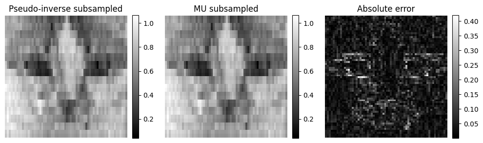
Again, in this setup, nonnegativity alone is essentially useless, since the subsampled pseudo-inverse reconstruction is already nonnegative. This means that the reconstruction error for both the regularized least squares and the MAP is null at \(\hat{X} = A^{\dagger}y\); both reconstructions may provide the exact same estimate. Moreover, we see on the error map that the original image is poorly estimated around the edges. This observation is consistent with the absence of high-frequency content. The image details cannot be reconstructed solely from the measurements.
Unmixing and reconstruction with known spectra and nonsmooth priors#
Joint reconstruction and unmixing principle#
As discussed in the introduction of this section, when considering hyperspectral images, it is reasonable to assume that the spectrum at each pixel is a linear combination of so-called endmembers, which are the spectra of pure materials present in the scene. When there are \(r\) different endmembers and \(r\) is smaller than the number of pixels \(n\) and the number of spectral bands \(p\), a simple but powerful model to represent the hyperspectral image is NMF,
where the nonnegative matrix \(V\in\mathbb{R}_+^{p\times r}\) contains the endmembers columnwise, and the nonnegative matrix \(U\in\mathbb{R}_+^{n\times r}\) contains the abundance maps, that is, the proportion of each material at each pixel. Because the illumination of the scene is not homogeneous spatially, and spectra may vary depending on other physical parameters such as the geometry of the scene, we refrain from assuming that the abundances sum to one pixelwise, but we assume that they are bounded by one elementwise.
In preliminary works, we have assumed that the endmembers \(V\) are known. The acquisition model then becomes
and our goal is to design a state-of-the-art reconstruction algorithm that estimates the abundances \(U\), therefore performing jointly the reconstruction of the hypercube and its spectral unmixing.
Joint reconstruction and unmixing in one step#
In [Hariga et al., 2024], a simple strategy to jointly reconstruct and unmix a single-pixel image was proposed, computing the MLE from Equation (16) with an alternating optimization algorithm, in this case alternating MU. The update rule for the spectra \(V\) is the same as detailled in Nonnegative regressions: NNLS and NNKL, and for \(U\) it can be obtained simply by 1) flattening the variables, 2) computing the classical MU rule and 3) folding the output into a matrix (see also [Févotte and Idier, 2011]). This yields after simplification
The code for the algorithm is slightly too complex to show here and is available in the tensorly_hdr package. A \(\ell_1\) regularization is added on both factors, which adds a constant term in the denominator of the update and helps control the dynamics of the factors, see Implicit regularization in rLRA.
Since the optimization problem
is jointly nonconvex, initialization is important. A viable optimization for simple unmixing problems is to first perform the reconstruction, for instance, solving a NNLS problem, then use a pure-pixel selection algorithm such as SNPA [Gillis, 2014] to initialize \(V\).
This procedure is illustrated below on, first, a synthetic exemple, and then on a real dataset acquired in CREATIS.
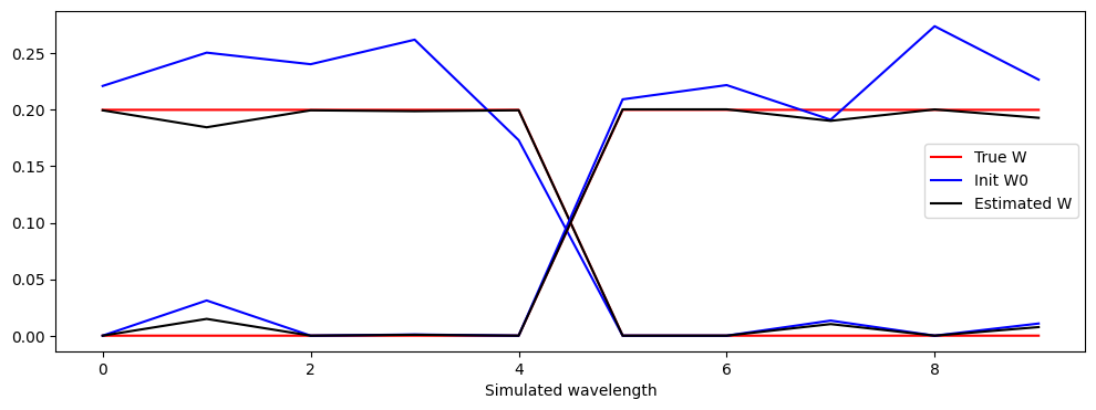
Synthetic experiment#
A dataset is generated in which two spectra have disjoint supports and lie on the boundary of the nonnegative orthant. This way, the NMF decomposition may be unique. Moreover, the abundances are designed to include pixels that are almost pure. No noise is added. We can observe that the reconstruction is good, but not perfect; this is mostly due to the non-uniqueness of the NMF model (which would require sparse abundances).
# Separation on synthetic dataset (Eusipco + HCERES)
import numpy as np
from tensorly_hdr.nmf_kl import MU_SinglePixel
from tensorly_hdr.sep_nmf import snpa

W = torch.tensor([[1,1,1,1,1,0,0,0,0,0],[0,0,0,0,0,1,1,1,1,1]], dtype=torch.float32).T
W = W/torch.sum(W, dim=0, keepdim=True)  # normalize columns
n = 32
At = torch.rand(2, n**2)
At = At/tl.sum(At,axis=0)
At[0,0]=0.99
At[1,1]=0.99
At[0,1]=0.01
At[1,0]=0.01
# Measurement operator is Ar, noiseless
Xtrue = W@At
alpha=1e2
meas_op = HadamSplit2d(n, noise_model=Poisson(alpha))  # this creates the split measurement operator A, and defines the model parameters (noise level)
Ar = torch.cat([meas_op.A[0:1,:], meas_op.A[2:,:]], dim=0) # TODO: adapt to use forward with wavelengths
Y = torch.poisson(alpha*Xtrue@Ar.T)
#Y = meas_op.forward(Xtrue)  # This sampled y~P(\alpha Ax)
Y = Y/alpha  # rescale to get back the right intensity scale

# Init pinv+spa
#X_rec = torch.linalg.lstsq(Ar, Y.T).solution.T
X_rec = hals_nnls(Ar.T@Y.T, Ar.T@Ar, n_iter_max=10).T
_, W0, A0 = snpa(X_rec, 2)

# Reconstruction with NMF
W_est, A_est, crit = MU_SinglePixel(Y, Ar, tl.abs(A0), tl.abs(W0), lmbd=0, maxA=None, niter=300, n_iter_inner=20, eps=1e-8, verbose=True, print_it=100)
# Normalization of W_est and A_est
sum_W_est = torch.sum(W_est, dim=0, keepdim=True)
W_est = W_est/sum_W_est
A_est = A_est*sum_W_est.T
Iteration 0, Cost: 91.79801177978516
Iteration 100, Cost: 91.32225036621094
Iteration 200, Cost: 91.1423568725586
Real data reconstruction and unmixing#
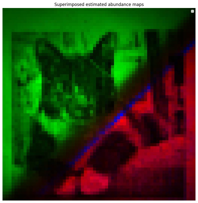
An acquisition was performed in the laboratory, with a cat image layered with two color filters, red and green. There is a thin spatial overlap between the two filters, which induces subtractive mixing; therefore, the hyperspectral image will be rank-two plus nonlinear mixing terms plus noise. However, the abundance maps are mostly disjoint, and the spectral bands where the green and red filters are intense also mostly do not overlap. Therefore, the separation problem is rather simple and amenable to separable NMF algorithms.
We first load the data and the metadata and process them to permute the acquisitions correctly. Then we remove the dark current, which is essentially the mean of the Gaussian noise in the Poisson-Gaussian mixture. We chose to ignore the Gaussian noise and assume that the only source of measurement variation is the Poisson distribution. However, Gaussian noise is not zero-centered, and the bias must be corrected. It can be estimated from the measurement acquired with the first row of the negative patterns \(H^{-}\), filled with zeros. The data is then clipped and normalized to lie in the interval \([0,1]\).
# Loading
import json
import ast

# Fetching the spectral measurements
data = np.load("../../tensorly_hdr/dataset/obj_Cat_bicolor_thin_overlap_source_white_LED_Walsh_im_64x64_ti_9ms_zoom_x1_spectraldata.npz", allow_pickle=True)
Ymeas = data["spectral_data"]

# Fetching metadata
file = open("../../tensorly_hdr/dataset/obj_Cat_bicolor_thin_overlap_source_white_LED_Walsh_im_64x64_ti_9ms_zoom_x1_metadata.json", "r")
json_metadata = json.load(file)[4]
file.close()

# replace "np.int32(" with an empty string and ")" with an empty string
tmp = json_metadata["patterns"]
tmp = tmp.replace("np.int32(", "").replace(")", "")
patterns = ast.literal_eval(tmp)  # the list (of list of) of pattern indices (evaluation because stored as text)
wavelengths = ast.literal_eval(json_metadata["wavelengths"])

# Permutation of measurements, that are acquired in an experiment-specific order
from spyrit.misc import sampling as samp
img_size = 64
acq_size = img_size
Ord_acq = (-np.array(patterns)[::2] // 2).reshape((acq_size, acq_size))
Ord_rec = torch.ones(img_size, img_size)
Perm_rec = samp.Permutation_Matrix(Ord_rec)
Perm_acq = samp.Permutation_Matrix(Ord_acq).T
Ymeas = samp.reorder(Ymeas, Perm_acq, Perm_rec)


# Post-processing of the measurements
Y = torch.tensor(Ymeas, dtype=torch.float32).T
del Ymeas

# Unbiased by removing the dark current, estimated as the minimum value of marginals of Y (better?)
dc = tl.sum(Y[:,1])/Y.shape[0] # average of dc over all wavelengths
print(f"Estimated dark current to remove: {dc}")
Y = Y - dc
Y = tl.clip(Y, 0, tl.max(Y))
# Normalization to [0,1]
Y = Y / tl.max(Y)

# Showing the measurements after dark current removal
plt.figure(figsize=(10,5))
plt.imshow(Y.cpu().numpy(), aspect='auto', cmap='gray')
plt.title("Measurements after dark current removal")
plt.xlabel("Pattern index")
plt.ylabel("Wavelength index")
plt.colorbar()
plt.show()
Estimated dark current to remove: 688.939453125
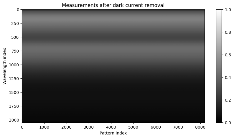
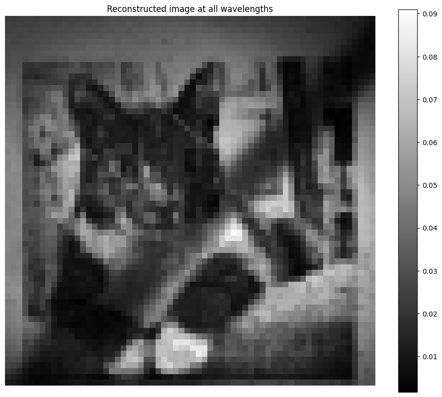
We then follow the reconstruction procedure described earlier. We remove some elements from the data matrix: the measurement with the row of zeros, which, apart from the dark current estimation, is uninformative, and some spectral bands that acquired no signal; here, the first 16 bands. The remaining spectral bands are binned into groups of size eight to reduce the dimension of the problem due to runtime issues. We first show here the pseudo-inverse reconstruction.
# Reconstruction with pseudo-inverse
from spyrit.core.meas import HadamSplit2d
import spyrit.misc.sampling as samp

# Patterns are acquired in order Acq, compared to order nat
# Patterns are stored in order Rec in spyrit
acq_size = img_size
meas_op = HadamSplit2d(img_size)
A = meas_op.A  # noiseless operator
Anz = torch.cat([A[0:1,:], A[2:,:]], dim=0)
print(Anz.shape)

# Remove row of zero and remove 16 first bands that are null
nbremove = 16
Ynz = torch.cat([Y[nbremove:,0:1], Y[nbremove:,2:]], dim=1)
wavelengths_nz = wavelengths[nbremove:]
print(f"Measurements shape after removing zero rows and first 16 bands: {Ynz.shape}")
# five bands binning
bin_size = 8
Ynz_binned = tl.zeros((Ynz.shape[0]//bin_size, Ynz.shape[1]))
wavelengths_binned = []
for i in range(0, Ynz.shape[0], bin_size):
    if i+bin_size <= Ynz.shape[0]:
        Ynz_binned[i//bin_size,:] = tl.mean(Ynz[i:i+bin_size,:], axis=0)
        wavelengths_binned.append(np.mean(wavelengths_nz[i:i+bin_size]))
    else:
        Ynz_binned[i//bin_size,:] = tl.mean(Ynz[i:,:], axis=0)
        wavelengths_binned.append(np.mean(wavelengths_nz[i:]))
Ynz = Ynz_binned
wavelengths_nz = wavelengths_binned
print(f"Binned measurements shape: {Ynz.shape}")

# define custom forward and adjoint forward functions
def forward(x):
    # x@Anz.T or Anz@x
    # x is of shape (B, N**2)  # batch first
    # reshape to (B, N, N)
    temp = x.reshape((x.shape[0], img_size, img_size))  # Whyyyyyyy >????
    temp = meas_op.forward(temp).T  # shape (M, B)
    # Removing the zero row of A changes the forward A@X
    return torch.cat([temp[0:1,:], temp[2:,:]], dim=0)
def adjoint(y):
    # Also implemented as a contraction in spyrit
    return y@Anz

# Pseudo-inverse reconstruction, the NNLS is quite slow here
X_rec = torch.linalg.lstsq(Anz, Ynz.T).solution.T

# Show cat reconstructed with all wavelengths
plt.figure(figsize=(12,10))
plt.imshow(np.rot90(torch.sum(X_rec, dim=0).reshape(64,64), 2), cmap='gray')
plt.title("Reconstructed image at all wavelengths")
plt.colorbar()
plt.axis('off')

plt.show()
torch.Size([8191, 4096])
Measurements shape after removing zero rows and first 16 bands: torch.Size([2032, 8191])
Binned measurements shape: torch.Size([254, 8191])
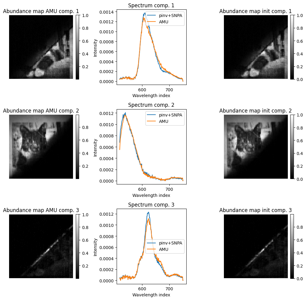
We now perform the pure-pixel selection and reconstruct/unmix jointly with an alternating MU algorithm. Observe how the abundance maps are well estimated with both methods, but the spectra are slightly smoother with the alternating MU algorithm. The third component (and in fact, most other components if the rank is increased) models the border of the overlap zone between the filters, which is intense because at the center of the image, and is not well modeled by a linear combination of the two filter spectra.
# Init pinv+spa
rank = 3
Kset, W0, A0 = snpa(X_rec, rank, verbose=True)

# Reconstruction with NMF
from tensorly_hdr.nmf_kl import MU_SinglePixel_fast
lmbd = 1e-4
W_est, A_est, crit = MU_SinglePixel_fast(Ynz, forward, adjoint, tl.abs(A0), tl.abs(W0), lmbd=lmbd, maxA=1, niter=60, n_iter_inner=20, eps=1e-8, verbose=True, print_it=20)  # regularization just for implicit scaling
print("Computation done")
0 [0, 0, 0]
1 [1688, 0, 0]
2 [1688, 2547, 0]
Returning [1688, 2547, 1816] as estimated pure pixel indices
Iteration 0, Cost: 3.21842360496521
Iteration 20, Cost: 3.1692192554473877
Iteration 40, Cost: 3.1318042278289795
Computation done
/tmp/ipykernel_2903/325737463.py:14: DeprecationWarning: __array_wrap__ must accept context and return_scalar arguments (positionally) in the future. (Deprecated NumPy 2.0)
  plt.plot(wavelengths_nz, A0norms[i]*W0[:,i].cpu().numpy())
/tmp/ipykernel_2903/325737463.py:15: DeprecationWarning: __array_wrap__ must accept context and return_scalar arguments (positionally) in the future. (Deprecated NumPy 2.0)
  plt.plot(wavelengths_nz, Anorms[i]*W_est[:,i].cpu().numpy())