
Automatic music transcription#
Reference
[Wu et al., 2022] H. Wu, A. Marmoret and J. E. Cohen, “Semi-Supervised Convolutive NMF for Automatic Music Transcription”, SMC2022, pdf code data
Nonnegative matrix factorization for automatic music transcription#
Spectrograms of piano recordings contain the spectral information of the notes played over time. An interesting property of the spectrogram of a single piano note recording is that it is typically well approximated by a rank-one matrix. For instance, on a recorded piano A4 (440Hz) from the dataset MAPS [Emiya et al., 2010], the best rank-one approximation of the magnitude spectrogram looks similar to the magnitude spectrogram, in particular when using KL-divergence as a loss function, see the end of the section on NNLS for a discussion on the rank-one approximation closed-form algorithm.
from cmath import phase
import matplotlib.pyplot as plt
import soundfile as sf
import numpy as np
import scipy.signal as signal

A4_wav, sr = sf.read('../../tensorly_hdr/dataset/MAPS_ISOL_LG_M_S0_M69_ENSTDkAm.wav')
A4_wav = A4_wav / np.max(np.abs(A4_wav)) # audio normalization
A4_wav = A4_wav[:,0] # use only one channel if stereo

# Compute spectrogram
frequencies, times, Sxx = signal.stft(A4_wav, fs=sr, nperseg=4096, nfft=4096, noverlap=4096 - 882)
half_freqs = len(frequencies) // 2
frequencies = frequencies[:half_freqs]
Sxx = Sxx[:half_freqs, :] # keep only lower half
Sphase = np.angle(Sxx)
Sxx_dB = 20 * np.log10(np.abs(Sxx) + 1e-10)  # convert to dB scale
Sxx_abs = np.abs(Sxx)

# Best rank-one approximation of magnitude spectrogram in the Frobenius sense
U,s,V = np.linalg.svd(Sxx_abs)
r1_approx = s[0]*np.outer(U[:,0],V[0,:])
# in dB
r1_approx_dB = 20 * np.log10(r1_approx + 1e-10)
# Same in KL sense with NMF
ukl = np.sum(Sxx_abs, axis=1)/np.sqrt(np.sum(Sxx_abs))
vkl = np.sum(Sxx_abs, axis=0)/np.sqrt(np.sum(Sxx_abs))
r1_approx_kl = np.outer(ukl, vkl)

r1_approx_kl_dB = 20 * np.log10(r1_approx_kl + 1e-10)
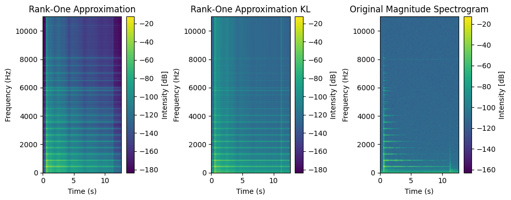
Magnitude spectrograms are rather well approximated by rank-one matrices. This suggests using low-rank NMF to analyse recordings containing multiple notes. Assuming a linear additive mixture of time signals, however, does not yield an exact low-rank model of the magnitude spectrogram, as explained next.
Simplified model and low-rank spectrograms#
Assume two notes are played simultaneously by the piano, with time signals \(s_1(t)\) and \(s_2(t)\). We focus on a single time window in the STFT. We assume linear mixing, and record the sum of the two signals \(s(t) = s_1(t) + s_2(t)\). The Fourier transform of the summed signal \(\mathcal{F}[s](\nu)\), by linearity of the Fourier transform, is exactly \( \mathcal{F}[s_1](\nu) + \mathcal{F}[s_2](\nu) \).
As we saw in Applications of rLRA: summary, the phase of the spectrogram is not low-rank even for a single note, therefore we only want to compute the magnitude spectrogram \(\left| \mathcal{F}[s] (\nu)\right| \), where the modulus is taken elementwise. However if we assume that \(\left|\mathcal{F}[s_{i}](\nu)\right|\) are rank-one matrices, we find that
and by Cauchy-Schwartz, the spectrogram computed from the recording is rank-two if and only if \( \mathcal{F}[s_1](\nu) = \lambda_\nu \mathcal{F}[s_2](\nu) \) for each \(\nu\) and \(\lambda_nu\geq 0\). This condition is equivalent to assuming that the two signals are in phase, i.e., \(\mathcal{Im}\left(\mathcal{F}[s_1]^\ast(\nu) \mathcal{F}[s_2](\nu)\right)=0\).
A particular case of the equality condition in Cauchy-Schwartz is obtained when the two frequency spectra have disjoint support, in which case \(\lambda_\nu\) is null. In other words, if the notes \(s_1(t)\) and \(s_2(t)\) have no partials in common, then the spectrogram of their additive mixture in the temporal domain should remain low-rank, and one can hope to recover each rank-one spectrogram by performing a rank-two NMF. This assumption is related to time-frequency masking, a technique that has been used for decades in audio source separation and has remained in use at the start of the era of deep learning [Araki et al., 2025].
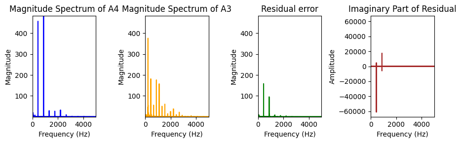
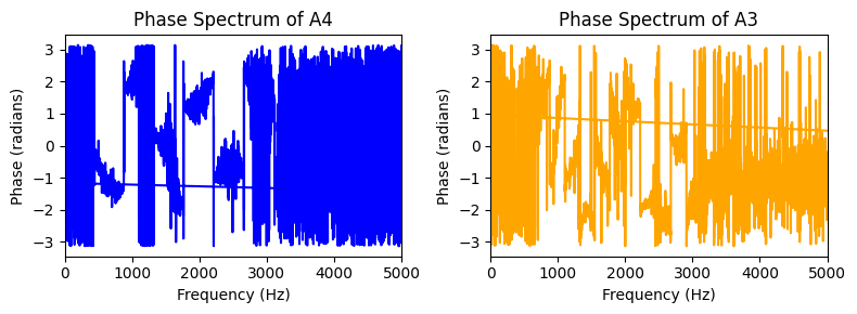
The disjoint support hypothesis is useful, but incorrect in practice. For instance, two notes separated by an octave have similar spectra, but the colinearity condition will be significantly violated. Not only are the fundamental frequencies and partials different in amplitude, but the phase of each signal can also change. This can be observed on the MAPS dataset below with notes A4 and A3. Observe that the imaginary part of the cross product is, in particular, nonzero at locations where the sum of the modulus is far from the modulus of the sum, and that this corresponds to partials of interest. This implies that methods based on low-rank approximations of spectrograms are particularly prone to octave errors.
from cmath import phase
from re import A
import matplotlib.pyplot as plt
import soundfile as sf
import numpy as np
import scipy.signal as signal

A3_wav, sr = sf.read('../../tensorly_hdr/dataset/MAPS_ISOL_LG_F_S1_M57_ENSTDkAm.wav')
A4_wav, sr = sf.read('../../tensorly_hdr/dataset/MAPS_ISOL_LG_M_S0_M69_ENSTDkAm.wav')
A4_wav = A4_wav / np.max(np.abs(A4_wav)) # audio normalization
A4_wav = A4_wav[:,0] # use only one channel if stereo
A3_wav = A3_wav / np.max(np.abs(A3_wav)) # audio normalization
A3_wav = A3_wav[:,0] # use only one channel if stereo
# Use short time window (rectangular window for simplicity)
t_1 = 2*sr
t_2 = 3*sr
A4_segment = A4_wav[t_1:t_2]
A3_segment = A3_wav[t_1:t_2]

# Compute 1D Fourier transform
frequencies_1D = np.fft.fftfreq(len(A4_segment), d=1/sr)
fourier_1D_A4 = np.fft.fft(A4_segment)
fourier_1D_A3 = np.fft.fft(A3_segment)
magnitude_1D_A4 = np.abs(fourier_1D_A4)
phase_1D_A4 = np.angle(fourier_1D_A4)
magnitude_1D_A3 = np.abs(fourier_1D_A3)
phase_1D_A3 = np.angle(fourier_1D_A3)

# Compute sum of magnitude and magnitude of sum
fourier_sum = fourier_1D_A4 + fourier_1D_A3
magnitude_sum = np.abs(fourier_sum)
fourier_magnitude_sum = magnitude_1D_A4 + magnitude_1D_A3
Note
AMT entered the MIREX competition as polyphonic transcription in 2024 (in fact, it was just piano, not guitar, organs, synthesizers, or others), even though it was already a research topic in the early 2000s. Single-instrument transcription remains an open problem, and there is much to do in a multi-instrument setting, particularly for joint source separation with AMT.
NMF for AMT: useful but limited#
Given a spectrogram \(Y\) of an audio recording, based on the observation that individual notes have approximately rank-one spectrograms, and assuming both linear mixture and marginally overlapping support of the spectrograms, one may hope to recover each individual note spectrogram with NMF. In fact, if the supports of the spectrograms of each note do not overlap, NMF is separable (each row of the data spectrogram belongs to exactly one note spectrogram), and therefore, the unique NMF solution can be recovered by any reasonable NMF algorithm. On top of estimating each individual spectrogram, these spectrograms are factorized into a temporal activation, which indicates when each note is played and at what intensity, and a frequency spectrum containing the fundamental and partials characteristic of the note. A simple post-processing step thus involves identifying the fundamental frequency for each rank-one NMF component, and thresholding the time-activation [Vincent et al., 2008]. Although more elaborate strategies could be designed, this pipeline is essentially what has been used in the AMT literature to post-process NMF factors.
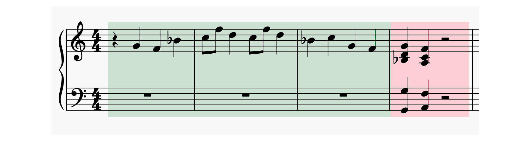
Fig. 34 Symbolic notation for the recorded audio sample. In green, the first six seconds with isolated notes, and in red, the second part, up to eight seconds, with chords.#
We can try this on a simple recording from the MAPS dataset [Emiya et al., 2010] with many isolated notes and few chords. The first example below is performed on a song with only isolated notes (first three bars). Notice how good the reconstruction is. There are six distinct notes played in the first six seconds of the recording. We used a rank seven NMF. One of the component models the hammer action; this can be seen by the spectral signature, which is not comb-shaped, and the time activation following each played note, except the high F, which has a softer attack.
# Load song
song, sr = sf.read('../../tensorly_hdr/dataset/MAPS_MUS-muss_1_ENSTDkAm.wav')
song = song / np.max(np.abs(song)) # audio normalization
song = song[:,0] # use only one channel if stereo
# The song has six different single notes until 6s, then chords
# We cut the song after 6s (rectangular window for simplicity)
t_1 = 0*sr
t_2 = 6*sr
song = song[t_1:t_2]

# Compute spectrogram
frequencies, times, Sxx = signal.stft(song, fs=sr, nperseg=4096, nfft=4096, noverlap=4096 - 882)
half_freqs = len(frequencies) // 2
frequencies = frequencies[:half_freqs]
Sxx = Sxx[:half_freqs, :] # keep only lower half
Sxx_dB = 20 * np.log10(np.abs(Sxx) + 1e-10)  # convert to dB scale
Sxx_abs = np.abs(Sxx)

# NMF with KL divergence (function taken from paper with Quyen, using alternating MU, code from tensorly_hdr)
# Could also use spa or snpa on the rows
from tensorly_hdr.nmf_kl import Lee_Seung_KL
rank = 7
np.random.seed(0)  # for reproducibility
W_init = np.abs(np.random.randn(Sxx.shape[0], rank))
H_init = np.abs(np.random.randn(Sxx.shape[1], rank)).T
crit, W_kl, H_kl, toc, cnt = Lee_Seung_KL(Sxx_abs, W_init, H_init, NbIter=20, verbose=False, print_it=20)
# Normalize W columnwise and put the norm in H
W_kl_norms = np.max(W_kl, axis=0)
W_kl = W_kl / W_kl_norms
H_kl = H_kl.T * W_kl_norms

# Permuting spectra in increasing fundamental frequency
from tensorly_hdr.image_utils import permute_spectra
perm = permute_spectra(W_kl)
W_kl = W_kl[:, perm]
H_kl = H_kl[:, perm]
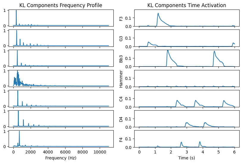
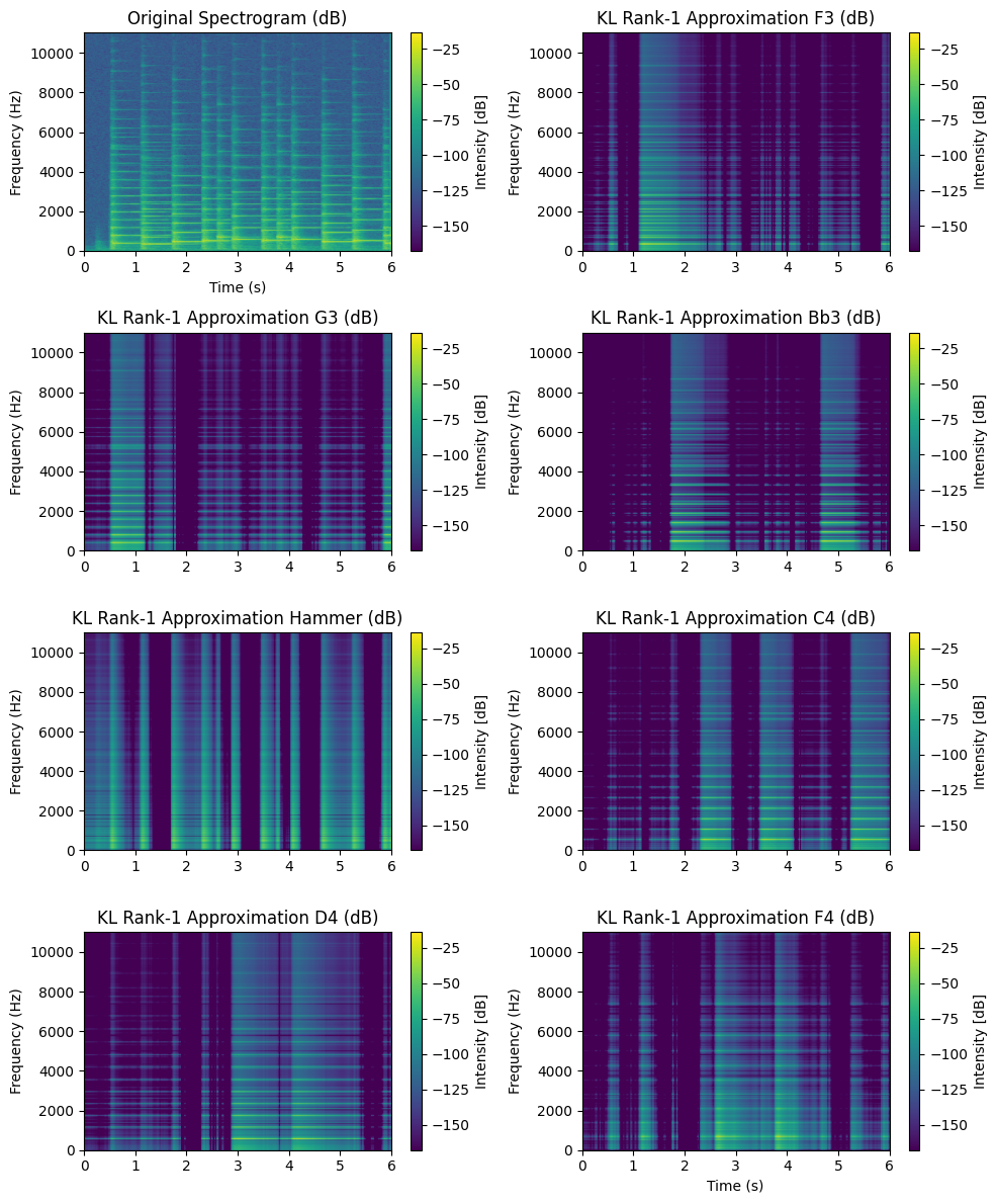
While this is promising, we knew the correct number of notes in the recording. Also, the rank-one spectrograms are not well located in time when analyzed on a logarithmic scale. For instance, the spectrogram of C4 has small but nonzero values when all the other notes are played.
Adding the next few seconds makes things much harder to analyse. The audio contains two chords, each with five notes, for a total of 14 distinct notes played. We see in the experiment below that NMF-KL does not identify all the notes. Instead, it introduces components to refine its approximation of the already identified notes.
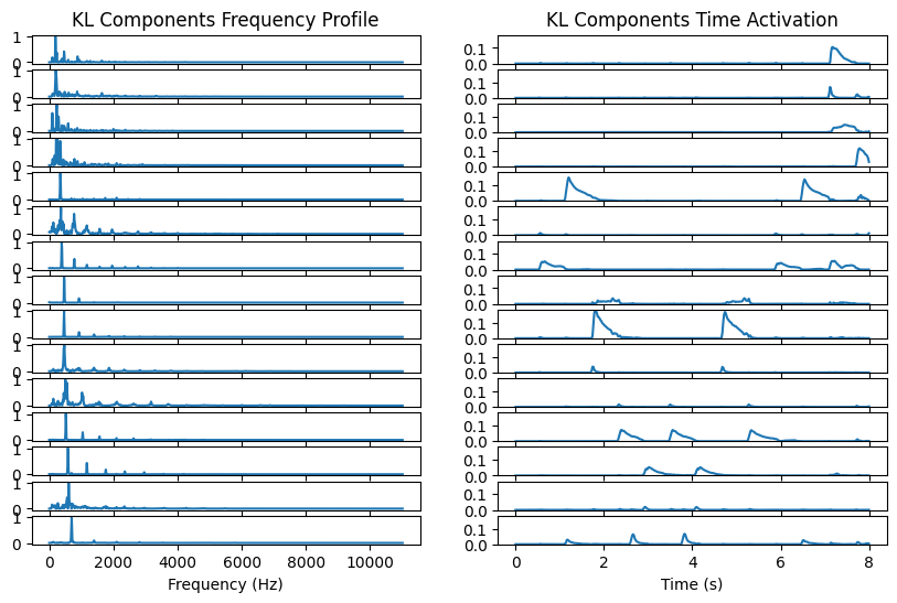
This suggests a few problems with NMF:
The rank-one hypothesis for isolated notes is not good enough. Therefore, the model tends to use several components to model a single note. This makes the choice of the rank harder, and the post-processing also more challenging.
We have little guarantee that the output spectra are indeed interpretable as comb-like spectra with a clear fundamental frequency. We clearly see in the above example that the components with the smallest fundamental frequency are hardly interpretable. Their time activation is also far from the standard attack-hold-sustain-decay pattern. In other words, the uniqueness of NMF is unclear as soon as many notes overlap in time and frequency, which is usually the case with chords in tonal music.
Tentative improvements to blind NMF for AMT involve parameterizing the time activations to actually follow and attack-decay pattern [Cheng et al., 2016]. We used a different route and utilized the so-called Convolutive NMF with supervision.
Convolutive pretrained NMF for improved piano transcriptions#
In [Wu et al., 2022], we proposed to address both issues: the modeling errors of spectrograms of single notes are reduced by introducing convolutive rank-one components, while the interpretability is ensured by pretraining the dictionary \(W\) on isolated notes recordings, thus switching from an unsupervised setup to a (weakly) supervised framework. Let us first discuss convolutive NMF.
Convolutive NMF, a better model for notes spectrograms#
As mentioned in Applications of rLRA: summary, magnitude spectrograms of single piano notes are not exactly rank-one matrices. While it is rather accurate that a single activation vector can describe the dynamics of the note over time, the description of a single note as a fixed frequency spectrum is wrong. The spectrum near the attack contains transients that rapidly dissipate. It therefore may differ significantly from the spectrum measured when the note is sustained. Ideally, to obtain a linear model, we could split attack and decay/sustain spectra as proposed in [Cheng et al., 2016]. We proposed to model each single note spectrogram \(Y[f,t]\) as the convolution of a small time-frequency matrix with a time activation:
where \(T\) is the size of the convolution window. This rank-one convolutive model can also be seen as a constrained rank \(T\) NMF if we consider the Toeplitz matrix \(\tilde{H}\) obtained by stacking rows of \(h\) shifted by one:
Convolutive NMF is obtained by modeling a nonnegative matrix as the sum of rank-one convolutive terms as defined in (15), that now depend on the component index \(q\). It was proposed originally in the context of speech separation [Smaragdis, 2006], and writes
The figure below compares NMF and CNMF on a visual example.
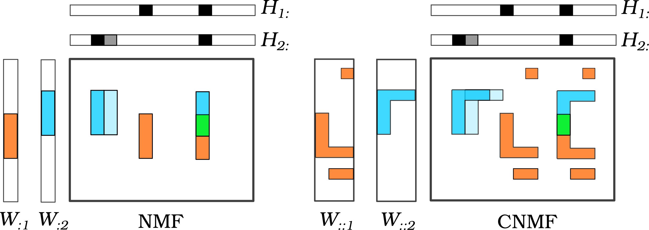
Fig. 35 Illustration of the CNMF model compared to NMF.#
Computing CNMF is typically done in an alternating fashion. Here, we do not need the full update of the tensor \(W\) in CNMF, since we will only use rank-one CNMF during training. The update for \(H\) provided in the original CNMF paper is a heuristic, but it was later refined using majorization-minimization techniques [Fagot et al., 2019] similar to what we describe in Nonnegative regressions: NNLS and NNKL. In terms of optimization, multiplicative update rules for CNMF are obtained essentially with the same majorization techniques as introduced in Nonnegative regressions: NNLS and NNKL. Indeed, the MU algorithm relies on a majorization that removes the dependence of each variable on the others, and, in that respect, CNMF has the same structure as NMF. The updates for tensor \(W^{(k)}\) and matrix \(H^{(k)}\) and iteration \(k\) can be written in matrix format as follows (following the MM2 algorithm from [Fagot et al., 2019]):
where \(\hat{Y}\in\mathbb{R}^{m\times n}\) is the reconstructed dataset, matrix \(\tilde{H}\) is computed from matrix \(H\) by shifting each row \(T\) times and concatenating the results, resulting in a block-Toeplitz matrix. Recall that \(\times_{1,2}\) denotes the tensor contraction on modes 1 and 2, and here corresponds to the broadcasted inner product of slices of \(\frac{Y}{\hat{Y}}\) with each slice of tensor \(W\) along the third mode. Zero-padding can be considered to handle the border of the input spectrogram.
Similarly to NMF, CNMF is a nonconvex problem. Personal observations lead me to believe that CNMF is significantly harder, with many non-trivial local minima, and therefore initialization is crucial.
A CNMF dictionary of pure notes with rank-one CNMF#
Armed with the iterative algorithm we just described, we can decompose the spectrogram of a single note, say A4, with rank-one CNMF. The template tensor \(W\), which has a single slice for rank-one CNMF and is therefore essentially a matrix, is initialized by copying the slice of the input spectrogram \(Y[:,t_0-3:t_0-3+T]\) where \(t_0\) is the index of the maximum column in \(\ell_1\) norm, and \(T\) is set to 10. This corresponds to selecting the most intense 0.2 seconds of the input spectrogram. This way, we ensure that the CNMF template is interpretable as a part of the spectrogram of A4. Random initialization may lead to a smaller loss function at convergence, but the results are harder to interpret. Separable CNMF has been studied in the literature [Degleris and Gillis, 2020].
A4_wav, sr = sf.read('../../tensorly_hdr/dataset/MAPS_ISOL_LG_M_S0_M69_ENSTDkAm.wav')
A4_wav = A4_wav / np.max(np.abs(A4_wav)) # audio normalization
A4_wav = A4_wav[:,0] # use only one channel if stereo
# Work on the first few seconds to avoid learning the recording noise around 10s
A4_wav = A4_wav[sr//3:sr*4]
# Compute spectrogram up to 10kHz
frequencies, times, Sxx = signal.stft(A4_wav, fs=sr, nperseg=4096, nfft=4096, noverlap=4096 - 882) #8192
# Cut for speed
half_freqs = len(frequencies) // 2
Sxx_dB = 20 * np.log10(np.abs(Sxx[:half_freqs,:]))  # convert to dB scale for display
Sxx_abs = np.abs(Sxx[:half_freqs,:])
# normalization
Sxx_abs = Sxx_abs / np.max(Sxx_abs)

# Testing rank-1 CNMF
T = 20
from tensorly_hdr.cnmf import convolutive_nmf
W_r1, H_r1, err_r1 = convolutive_nmf(
    Sxx_abs, rank=1, T=T, itmax=10, eps=1e-16, tol=0,
    print_it=1, n_iter_inner=10, init="separable", verbose=False
    )
W_cnmf=W_r1[:, :, 0]
h_cnmf = H_r1[0, :]
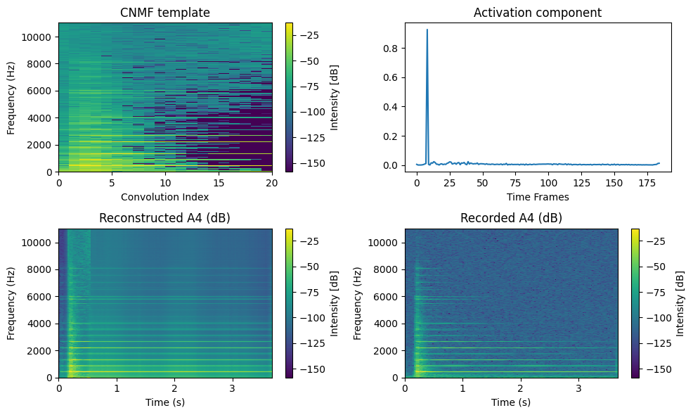
Observe that the time activation profile is sparser than with the best rank-one NMF approximation, which is expected since the template now contains short-time information. The template, however, has some issues. It captures correctly the attack spectrum with a comb-shaped spectrum and many harmonics, but the high-pitch harmonics should decrease in intensity. The content of the template after the attack above 4kHz is therefore not realistic.
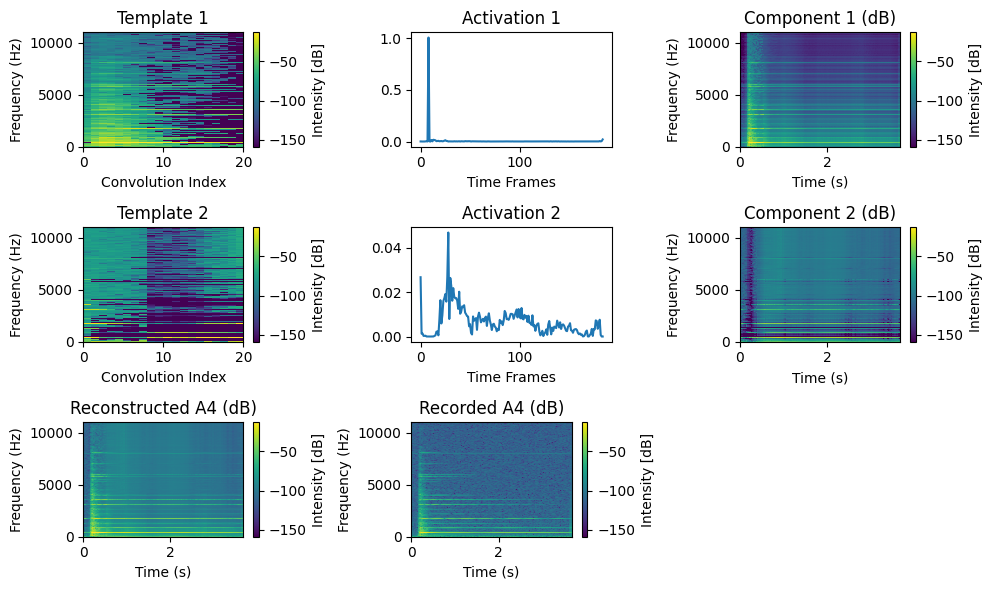
This problem appears to be due to the rank-one model modeling echoes observed in the signal. To alleviate this issue, one can compute a rank-two CNMF with the second template initialized randomly. Observe how this second component captures noise and high-frequency decay spectra, effectively cleaning the first component. In particular, the second component does not model the attack. For simplicity and computational speed reasons, we will work with rank-one CNMF approximations of single notes, as done in regular NMF.
W_r2, H_r2, err_r2 = convolutive_nmf(
    Sxx_abs, rank=2, T=T, itmax=10, eps=1e-16, tol=0,
    print_it=1, n_iter_inner=10, init="separable", verbose=False
    )
Transcription example on MAPS#
In this document, we simply provide a toy example of AMT with pretrained templates. Our goal is to transcribe the same audio recording as above with isolated notes and two chords. We know the notes utilized in the recording, and MAPS has all single notes recorded individually. Therefore, we can perform rank-one CNMF on each note recording, and then transcribe the recorded music.
import os
import re
import numpy as np
import soundfile as sf
from scipy import signal
from tensorly_hdr.cnmf import convolutive_nmf

# Directory with your .wav files
data_dir = '../../tensorly_hdr/dataset/notes_to_learn'
T = 10
rank = len(os.listdir(data_dir))  # 14

# Templates list
Wlist = []
names = []
display = ""

# Learning the templates
# perform the code below but with every file in ../../tensorly_hdr/dataset/notes_to_learn
for filename in os.listdir(data_dir):
    midi_num = re.search(r'M(\d+)_', filename).group(1)
    display += f"Processing MIDI note: {midi_num} \n"
    names.append(midi_num)
    filepath = os.path.join(data_dir, filename)
    A4_wav, sr = sf.read(filepath)
    A4_wav = A4_wav / np.max(np.abs(A4_wav)) # audio normalization
    A4_wav = A4_wav[:,0] # use only one channel if stereo
    # Work on the first few seconds to avoid learning the recording noise around 10s
    A4_wav = A4_wav[0:sr*4]

    # Compute spectrogram up to 10kHz
    frequencies, times, Sxx = signal.stft(A4_wav, fs=sr, nperseg=4096, nfft=4096, noverlap=4096 - 882) #8192
    # Cutting last few time frames (40ms) because there are artifacts (probably from the windowing above)
    Sxx = Sxx[:,:-2]
    times = times[:-2]
    half_freqs = len(frequencies) // 2
    Sxx_dB = 20 * np.log10(np.abs(Sxx[:half_freqs,:]))  # convert to dB scale
    Sxx_abs = np.abs(Sxx[:half_freqs,:])
    # normalization
    Sxx_abs = Sxx_abs / np.max(Sxx_abs)

    # rank-1 CNMF
    # Only init
    W_r1, H_r1, err_r1 = convolutive_nmf(Sxx_abs, rank=1, T=T, itmax=10, eps=1e-16, tol=0, print_it=10, n_iter_inner=10, init="separable", verbose=False)
    Wlist.append(W_r1[:, :, 0])
    h_cnmf = H_r1[0, :]
    display += f"Reconstruction error: {err_r1[-1]} \n"
print(display)

# Post-process Wlist into a tensor
W = np.zeros((Wlist[0].shape[0], Wlist[0].shape[1], rank))
for r in range(rank):
    W[:, :, r] = Wlist[r]

# Permute by increasing MIDI name
perm = np.argsort(names)
names = np.sort(names)
W = W[:,:,perm]
names_music = ["G2", "A2", "F3", "G3", "A3", "Bb3", "C4", "D4", "F4", "G4", "Bb4", "C5", "D5", "F5"]
Processing MIDI note: 55
Reconstruction error: 19.834237201753123
Processing MIDI note: 45
Reconstruction error: 30.93537125880311
Processing MIDI note: 72
Reconstruction error: 29.097904149414045
Processing MIDI note: 65
Reconstruction error: 13.32250937482522
Processing MIDI note: 58
Reconstruction error: 35.91304523687367
Processing MIDI note: 67
Reconstruction error: 60.52892755730625
Processing MIDI note: 77
Reconstruction error: 12.280582957024
Processing MIDI note: 62
Reconstruction error: 69.47470723043435
Processing MIDI note: 43
Reconstruction error: 45.81653411044577
Processing MIDI note: 70
Reconstruction error: 10.964860173074516
Processing MIDI note: 74
Reconstruction error: 28.32652578812197
Processing MIDI note: 57
Reconstruction error: 16.437007590423867
Processing MIDI note: 53
Reconstruction error: 39.798393135226604
Processing MIDI note: 60
Reconstruction error: 21.000479659714145
Now that the training is performed, we can transcribe the audio recording!
from tensorly_hdr.cnmf import convolutive_regression
H_tr, err = convolutive_regression(Sxx_abs, W, itmax=50, verbose=True, print_it=25)
Iteration initial, loss: 92399.14369493214
Iteration: 25, loss: 19.24762348839989
Iteration: 50, loss: 19.043476148742613
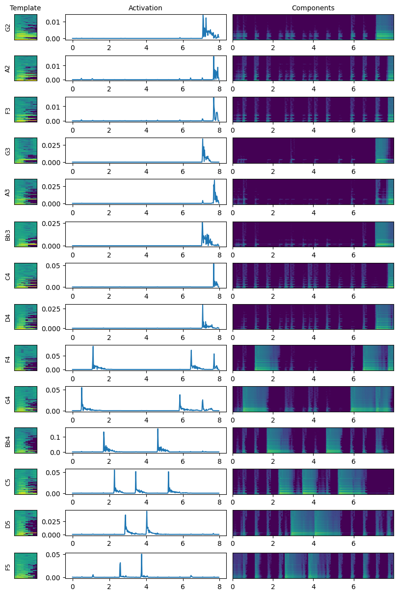
The song is now well transcribed. In particular, the last two chords have the right five notes, played simultaneously. The chord activations are still imperfect, but this is expected because of the non-linear mixing artifacts and the frequency similarity between octaves. We also see that all components slightly activate on each attack. This might be due to the hammer-action sound, which is the same across all notes and has not been taken into account separately.
The full model, weakly supervised on all piano notes, has performance close to that of fully supervised networks but is not robust to distribution shift (e.g., changing the piano or the recording conditions) [Wu et al., 2022]. Improving these aspects and the training procedure is part of my research project.