

Implementing NNLS - NNKL solvers#
In this lession, your goal is to
implement a NNLS/NNKL solver of your choice (AS, HALS, MU),
test is numerically on synthetic examples,
implement a NMF solver using alternating optimization.
You can start by choosing one type of loss function, either least squares
or Kullback-Leibler
Then choose one of the three algorithms seen in class:
MU is simpler, but slower for NNLS
HALS is moderately hard to implement, and fast for matrix problems
Active set is the hardest to implement (but also fun !)
Keep in mind that you will use this function with a matrix input when solving NNF later on.
Please refrain from generating all the code with AI tools (these algorithms are available online so it will copy paste the solution in seconds), but feel free to use it for debugging if you are stuck.
Packages you need: numpy (pip install numpy) tensorly (pip install tensorly)
import numpy as np

def MultiplicativeUpdatesLS(y,U,x0=None,maxiter=1000,tol=1e-6):
    """
    Multiplicative updates for least squares problem.

    Parameters:
    y : array-like, shape (n_samples,)
        The observed data vector.
    U : array-like, shape (n_samples, n_features)
        The design matrix.
    maxiter : int
        Maximum number of iterations.
    tol : float
        Tolerance for convergence.

    Returns:
    x : array-like, shape (n_features,)
        The estimated coefficients.
    loss: array-like, shape (maxiter,)
        The loss at each iteration.
    """
    # Initialize x with non-negative values
    if x0 is not None:
        x = x0.copy()
    else:
        x = np.random.rand(U.shape[1])  # does not work if matrix input
    loss = np.zeros(maxiter)
    Uty = U.T@y
    UtU = U.T@U
    for i in range(maxiter):
        # Update rule
        x_new = np.maximum(x * Uty / (UtU@x), 1e-8)  # Add small value to avoid division by zero

        # Check for convergence
        if np.linalg.norm(x_new - x) < tol:
            break

        loss[i] = np.linalg.norm(y - U@x_new)
        x = x_new

    return x, loss[:i+1]


# Multiplicative updates  (or import from scipy)
def KLloss(y,z, eps=0):
    summand = y*np.log(y/(z+eps)) + z - y
    return np.sum(summand.flatten())

from scipy.special import kl_div

def MultiplicativeUpdatesKL(y,U,x0=None,maxiter=1000,tol=1e-6):
    """
    Multiplicative updates for least squares problem.

    Parameters:
    y : array-like, shape (n_samples,)
        The observed data vector.
    U : array-like, shape (n_samples, n_features)
        The design matrix.
    maxiter : int
        Maximum number of iterations.
    tol : float
        Tolerance for convergence.

    Returns:
    x : array-like, shape (n_features,)
        The estimated coefficients.
    loss: array-like, shape (maxiter,)
        The loss at each iteration.
    """
    # Initialize x with non-negative values
    if x0 is not None:
        x = x0
    else:
        x = np.random.rand(U.shape[1])  # does not work if matrix input
    loss = np.zeros(maxiter)
    #Ut1 = np.sum(U.T, axis=1)
    Ut1 = U.T@np.ones_like(y)

    for i in range(maxiter):
        # Compute the current estimate of y
        y_hat = U @ x

        # Update rule
        x_new = np.maximum(x * (U.T @ (y/y_hat) )/ Ut1 , 0)  # Add small value to avoid division by zero

        # Check for convergence
        if np.linalg.norm(x_new - x) < tol:
            break

        loss[i] = KLloss(y, y_hat)
        x = x_new

    return x, loss[:i+1]

# HALS LS
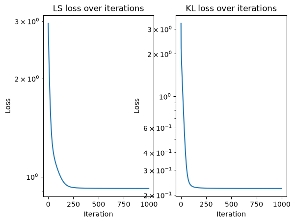
To test your algorithm, generate random nonnegative vectors \(x\) and nonnegative linear operators \(U\), then create synthetic examples of observations \(y\) according to a noise model that depends on the loss you chose.
Remember to introduce the hyperparameters explicitely (problem dimensions, noise level, number of iterations) so that you can easily play with them.
m, n = 100, 10
noise = 0.1
x = np.random.rand(n)
U = np.random.rand(m, n)
y = U @ x + noise * np.random.randn(m)  # Add some noise

# solver
out = MultiplicativeUpdatesLS(y, U, maxiter=1000, tol=1e-6)
out2 = MultiplicativeUpdatesKL(y, U, maxiter=1000, tol=1e-6)

# plotting loss
import matplotlib.pyplot as plt
plt.figure()
plt.subplot(1,2,1)
plt.semilogy(out[1])
plt.title('LS loss over iterations')
plt.xlabel('Iteration')
plt.ylabel('Loss')
plt.subplot(1,2,2)
plt.semilogy(out2[1])
plt.title('KL loss over iterations')
plt.xlabel('Iteration')
plt.ylabel('Loss')

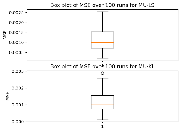
# Doing average MSE over 100 runs
n_runs = 100
mse_list = []
mse2_list = []

for _ in range(n_runs):
    x = np.random.rand(n)
    U = np.random.rand(m, n)
    y = U @ x + noise * np.random.randn(m)  # Add some noise
    out = MultiplicativeUpdatesLS(y, U, maxiter=1000, tol=0)
    out2 = MultiplicativeUpdatesKL(y, U, maxiter=1000, tol=0)
    mse = np.mean((x - out[0])**2)
    mse2 = np.mean((x -  out2[0])**2)
    mse_list.append(mse)
    mse2_list.append(mse2)

print(f'Average MSE: {np.mean(mse_list):.4f}')

# Box plot of the MSE
plt.figure()
plt.subplot(2,1,1)
plt.boxplot(mse_list)
plt.title('Box plot of MSE over 100 runs for MU-LS')
plt.ylabel('MSE')
plt.subplot(2,1,2)
plt.boxplot(mse2_list)
plt.title('Box plot of MSE over 100 runs for MU-KL')
plt.ylabel('MSE')
Average MSE: 0.0012
Text(0, 0.5, 'MSE')
Implementation of a NMF solver#
You can now use your NNLS/NNKL solver to implement an algorithm for computing an approximate NMF.
Keep in mind that iterative algorithms need initialization, and this is particularly important for NMF as it is nonconvex. A classical solution is to use the absolute value of SVD outputs. But you can also use separable NMF (code provided)
Another thing consider is the number of inner iterations of the NNLS/NNKL solvers. You can set this as an hyperparameter and compare various choices on a synthetic dataset.
from auxiliary_fun import spa

def NMF(Y, r, init=None, maxiter=1000, tol=1e-6, inner_maxiter=10, loss_type="LS"):
    """
    Non-negative Matrix Factorization using SPA for initialization and Multiplicative Updates for optimization.

    Parameters:
    Y : array-like, shape (n_samples, n_features)
        The data matrix to be factorized.
    r : int
        The rank of the factorization.
    init : tuple of array-like, optional
        Initial values for W and H. If None, SPA is used for initialization.
    maxiter : int
        Maximum number of iterations.
    tol : float
        Tolerance for convergence.

    Returns:
    W : array-like, shape (n_samples, r)
        The basis matrix.
    H : array-like, shape (r, n_features)
        The coefficient matrix.
    loss: array-like, shape (maxiter,)
        The loss at each iteration.
    """
    # initialization
    if init is not None:
        W, H = init
    else:
        _, W = spa(Y, r)
        H = np.random.rand(r, Y.shape[1])
    loss = np.zeros(maxiter)

    for i in range(maxiter):
        if loss_type=="LS":
            # Update H using Multiplicative Updates
            H, _ = MultiplicativeUpdatesLS(Y, W, x0=H, maxiter=inner_maxiter, tol=1e-6)

            # Update W using Multiplicative Updates
            Wt, _ = MultiplicativeUpdatesLS(Y.T, H.T, x0=W.T, maxiter=inner_maxiter, tol=1e-6)
            W = Wt.T

            # Compute the current estimate of Y
            Y_hat = W @ H

            # Compute loss
            loss[i] = np.linalg.norm(Y - Y_hat)**2

        elif loss_type=="KL":
            # Update H using Multiplicative Updates
            H, _ = MultiplicativeUpdatesKL(Y, W, x0=H, maxiter=inner_maxiter, tol=1e-6)

            # Update W using Multiplicative Updates
            Wt, _ = MultiplicativeUpdatesKL(Y.T, H.T, x0=W.T, maxiter=inner_maxiter, tol=1e-6)
            W = Wt.T

            # Compute the current estimate of Y
            Y_hat = W @ H

            # Compute loss
            loss[i] = KLloss(Y, Y_hat)

        # Check for convergence
        if i > 0 and np.abs(loss[i] - loss[i-1]) < tol:
            break

    return W, H, loss[:i+1]
To estimate the performance of your NMF algorithm, you can generate synthetic data as in the NNLS/NNKL problem. The issue is with measuring the error for \(W\) and \(H\) which suffer from scaling and permutation ambiguitees.
You can propose a solution to fix these ambiguitees, and compare your estimated solutions with the true ones. Because NMF may not be unique, mind that these solution may not match.
# Data generation
np.random.seed(0)
m, n, r = 100, 50, 5
W = np.random.rand(m, r)
H = np.random.rand(r, n)
Y = W @ H + np.random.uniform(0, 0.1, (m, n))

# NMF
W_est, H_est, loss = NMF(Y, r, maxiter=1000, tol=1e-6)
W_est_kl, H_est_kl, loss_kl = NMF(Y, r, maxiter=1000, tol=1e-6, loss_type="KL")

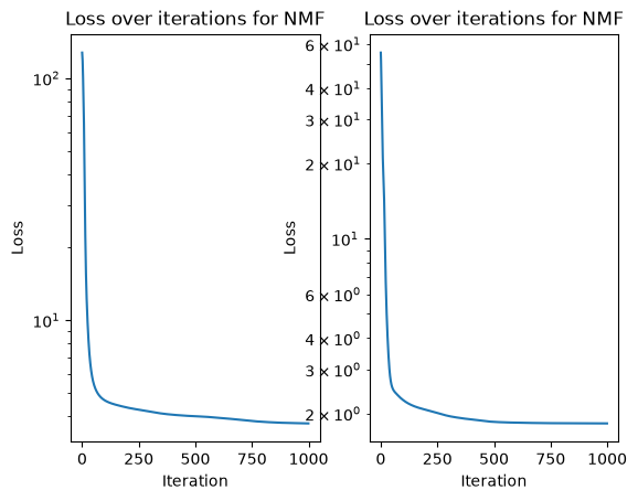
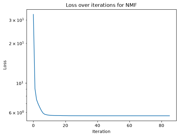
plt.figure()
plt.subplot(1,2,1)
plt.semilogy(loss)
plt.title('Loss over iterations for NMF')
plt.xlabel('Iteration')
plt.ylabel('Loss')
plt.subplot(1,2,2)
plt.semilogy(loss_kl)
plt.title('Loss over iterations for NMF')
plt.xlabel('Iteration')
plt.ylabel('Loss')
0 [0, 0, 0, 0, 0]
1 [19, 0, 0, 0, 0]
2 [19, 49, 0, 0, 0]
3 [19, 49, 49, 0, 0]
4 [19, 49, 49, 49, 0]
Returning [19, 49, 49, 49, 49] as estimated pure pixel indices
0 [0, 0, 0, 0, 0]
1 [19, 0, 0, 0, 0]
2 [19, 49, 0, 0, 0]
3 [19, 49, 49, 0, 0]
4 [19, 49, 49, 49, 0]
Returning [19, 49, 49, 49, 49] as estimated pure pixel indices
Text(0, 0.5, 'Loss')
On a real example#
We may now compute NMF on a real data example, anticipating on next lecture !
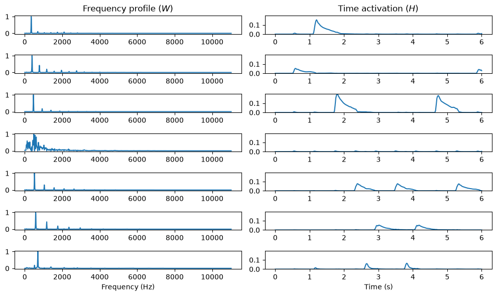
We will transcribe a simple piano recording, detailled explanations will be given tomorrow.
This requires installing two other packages: soundfile and scipy
import soundfile as sf
import scipy.signal as signal
from auxiliary_fun import permute_spectra

song, sr = sf.read('./MAPS_MUS-muss_1_ENSTDkAm.wav')  # loads data
song = song / np.max(np.abs(song))  # normalize the audio
song = song[:, 0]  # take left channel only
t_1, t_2 = 0, 6 * sr  # first six seconds: isolated notes only
song_simple = song[t_1:t_2]  # cut the first 6 seconds of the song for analysis
frequencies, times, Sxx = signal.stft(song_simple, fs=sr, nperseg=4096, nfft=4096, noverlap=4096 - 882)  # compute stft
half_freqs = len(frequencies) // 2  # keep right side of the spectrum only
frequencies = frequencies[:half_freqs]
Sxx = Sxx[:half_freqs, :]
Sxx_abs = np.abs(Sxx)

# hyperparameters
rank = 7
maxiter = 200
W_init = np.abs(np.random.randn(Sxx.shape[0], rank))
H_init = np.abs(np.random.randn(Sxx.shape[1], rank)).T

# insert your algorithm here
W_kl, H_kl, loss = NMF(Sxx_abs, rank, init=(W_init, H_init), maxiter=100, loss_type="KL")

W_kl_norms = np.max(W_kl, axis=0)
W_kl = W_kl / W_kl_norms
H_kl = H_kl.T * W_kl_norms

# Insert your postprocessing here
perm = permute_spectra(W_kl)

W_kl, H_kl = W_kl[:, perm], H_kl[:, perm]
# You can try and guess which note is which
#notes = ["F3", "G3", "Bb3", "Hammer", "C4", "D4", "F4"]

plt.figure(figsize=(10, 6))
for i in range(rank):
    plt.subplot(rank, 2, 2 * i + 1)
    plt.plot(frequencies, W_kl[:, i])
    #plt.ylabel(notes[i])
    if i == 0:
        plt.title('Frequency profile ($W$)')
    if i == rank - 1:
        plt.xlabel('Frequency (Hz)')
    plt.subplot(rank, 2, 2 * i + 2)
    plt.plot(times, H_kl[:, i])
    plt.ylim(0, np.max(H_kl))
    if i == 0:
        plt.title('Time activation ($H$)')
    if i == rank - 1:
        plt.xlabel('Time (s)')
plt.tight_layout()

plt.figure()
plt.semilogy(loss)
plt.title('Loss over iterations for NMF')
plt.xlabel('Iteration')
plt.ylabel('Loss')

plt.show()
If you have finished all the coding, you can try implementing another NNLS/NNKL solver and comparing them!